Earth, Migrations, and the Human Effect

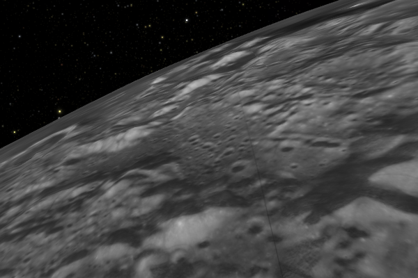
I want to take us back, all of us back, forty years ago this week. The last mission to the Moon. We’re flying up here at the altitude, we’re flying toward the landing site of Apollo 17. This is Taurus-Littrow Valley. A valley deeper than the Grand Canyon of Earth on a body one-quarter the size of Earth. These are data, we see a scene here, so come along.

But I wanted to take you back just to the very beginning of this. To the Moon to show you this comparison of the Moon that we worked so hard to get to forty years ago, on the last mission of Apollo 17. Gene Cernan and Jack Schmitt down on the Moon’s surface. And this is the crater Camelot. This is the landslide they drove up to. This is the half buried crater Nansen. And Shorty crater, which you can actually see downstairs in the lobby. And the mountains rimming Mare Crisium here and the dark lavas that flow out. This was the interesting area to go to.

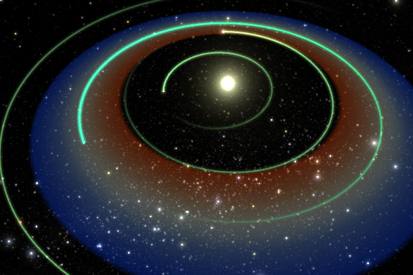
But after all the work going to the Moon, it was the Earth that we really focused on and looked back on. And so, with this, I wanted to just muse a little bit for us this cosmic context that we find ourselves within. As we come up on the solar system, this is the orbit of Pluto. This is Neptune, Uranus, Saturn, Jupiter, and then the inner planets of the solar system. We go around the Sun, so this shows you where the planet is and it’s trail orbiting back. And now I see the habitable zones. The Earth being in the middle, where it’s warm. Farther out to Mars, it’s colder. Farther in to Venus, unlivably warm. Closer to our star. And our Earth, up here, just at the, at the edge of its, its orbit that goes, been going around the Sun for almost five billion years. And the Earth formed about four-and-a-half billion years ago.

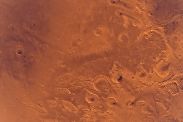
We’re coming up on the fourth planet of the solar system. Thinking back forty years into the past is, make sure this is (mumble), ok, that we come up on what looked like the future. Mars. And in 1971, we started to orbit Mars for the first time. We came into this desert-looking world. This is what Mars looks like through a telescope. Has a polar cap. Has atmosphere that we can see. But it’s a world half the size of Earth. And on this we can see what almost looked like the continental areas, but a reddish world. And in the mid-60’s, our first flights passed Mars, actually took us past craters, and it was later that we found the canyons of Mars, and so on. I still have my habitable zone down here, and it almost looks like a ring of Saturn. I’ll turn that off. But this is what Mars looked like on our first forays to this planet. And for an eleven-year-old, myself, and maybe some of you out there the same age when we flew to the Moon the last time, I certainly couldn’t let go the notion that maybe when I grew up we might go to Mars. And I know for some of the youngsters in the audience tonight, maybe, maybe one day you’ll set your, your feet on the soils of Mars. That Mars seemed like this great future on the way to the stars.

But when we look at this, let’s think back to the Moon, quarter of the size of Earth, cannot, does not have enough mass to hold an atmosphere. Mars, half the size of Earth, farther out in the colder reaches of the solar system, does have an atmosphere, a dusty atmosphere. It’s basically almost like talcum powder suspended in the atmosphere, local dust storms. When we got closer, we began to see these features that belied a history in the past that we now can (?) today using craters and so on, to see that these, these flowing channels of water that seem to scour and carve Mars, happened perhaps about three to three and a half billion years ago.

We’re entering the eastern reaches of the Valles Marineris, so called for the Mariner spacecraft, Mariner 9, that discovered this feature. Once again, Mars, being about half the size of the Earth, this canyon, however, would stretch from New York to Los Angeles. About a three thousand mile-long canyon. Unlike the flowing river area, as you saw earlier, that this feature seems to be a part of Mars that was stretching apart, and parts of the rock fell down, and this canyon has features that show that large landslides belie the geologic history of this. Also, in Candor Chasma, the widest section of Mars, we actually see that this area up here, of layered terrain. The only place where we know that layered terrain accumulates on Mars is at the pole. But this is near the equator. What happened on Mars?

Mars having a early epoch of, perhaps, water. Maybe life, since we know just of life on Earth, that life requires water. That we look to Mars, and scientifically Mars is a fantastic place to go to and look for the prospects of life having originated. And here, the labyrinth of night, we see the beginning of the canyon. And then the beginning of volcano country up here in the Tharsis Montes of these, some of the largest volcanoes in the solar system. And then, farther up to the northwest, we come to Olympus Mons. It’s the largest volcano in the solar system. It’s the size of New York state. It’s three times the height of Mount Everest. But in going to Mars, which, on a good day is, is basically still colder than Antarctica, we challenge ourselves in thinking, what is that future in taking life-support with us out into space to survive.

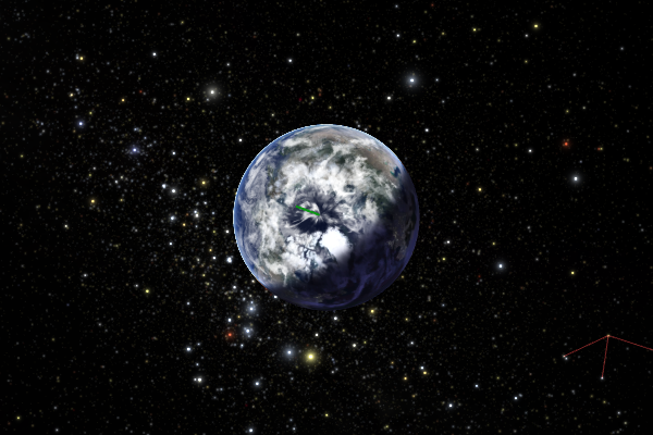
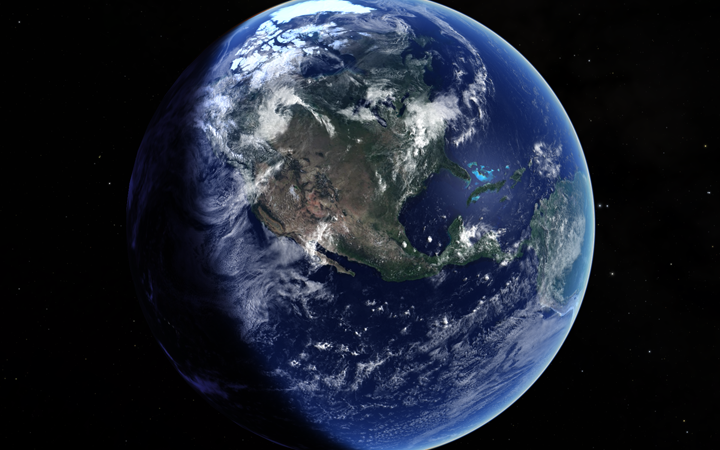
But looking at the solar system in this fashion, we begin to understand and appreciate that our planet itself, our planet Earth, is really in space. We spend all this time and money to, perhaps, go and send people to the Moon and eventually to Mars, is that we perhaps forget that we ourselves are in space. We’re coming up now on our Earth. This is the orbit of the Moon, a quarter million miles away. And now we see the continent of Australia. The fully illuminated, beautiful planet that we live on. And this is set to today, the 18th of December. It’s my mother’s 88th birthday. I couldn’t be with her. I’m here with you all tonight. But, it’s a great pleasure. We come around, we look at, right here, this is North America. These are the city lights. That’s Chicago. This is Florida. There we are, New York. This is California. And down is Mexico City.

We see the Sun as it’s crossing the Milky Way. It does this every year. It lines up with the Milky Way around the summer, or, sorry, around, well, summer solstice from the southern hemisphere. It’s winter solstice in the northern hemisphere. And the Earth rotates on an axis. This is Japan. Here’s Hong Kong. So we see Asia parading by. The Earth rotates. This is North Pole up here. And, here’s the Nile River. Here’s Italy. Here’s England. Here’s Paris. Here’s Madrid. And, United States once again.

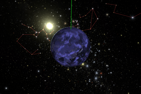
Let’s turn this a little faster. And as we proceed, we’re going to spin faster and faster on its axis. Might be a little dizzying, if you can kind of look to either side of Earth if you feel dizzy. But notice something is happening. Remember as we flew in I showed you how the orbits are delineated with the planets out ahead of their orbits. And we go around this star, the Sun. But to ride along with the Earth is to see the Sun moving against the zodiacal constellations which we turned on for you tonight. This is Sagittarius. That’s Capricorn. And this is Aquarius.

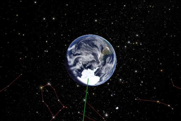
Let’s rotate along with the Earth. Earth, here just a little bit. Yeah. And, so just a second. We’re going to bring on the polar axis to show you. Here’s the spin axis. With Antarctica. And, you may notice, as Earth twirls kind of like a lollipop, notice this axis points up in this direction to this star. And that’s the North Star of which we really aim that with the Big Dipper. But, I moved this back so we can now see, at this time of year, how the North Pole is in night time. And the day-night cycle, here we see speeding time up, as we proceed. And we see the Sun move against constellations. Notice how the pole is come, starting to come in to light. Right about here. We’ll slow the Earth back down. We’ll show, this is the time of the, of the equinox. This is the vernal equinox. So, as the northern hemisphere starts to come into sun, let’s go down to Antarctica and see that it’s sort of half in shadow. So what was polar day, just sort of a quarter turn back around the Sun, is now becoming polar night. Whereas, or south polar night. North polar night is coming into day. So, as we spin, we can also see how, in this case we’re going to bring, we’re going to do this one more time. This is, I believe, Mercury and Venus. That’s probably Mercury right there. We can see these are the wandering stars, the planets, moving about. I think that’s Mars in the background perhaps.

We move the Sun as it’s now coming up to cross the Milky Way, the great circle of the Milky Way which, of course, is our galaxy. And, we look again. And, at this time, when the Sun is at its greatest northern reaches, we can see that to the North Pole is when the North Pole is illuminated and Antarctica is in night. And this diurnal cycle of rotation is what sets up the weather patterns that we understand on a daily pattern, and the seasons where I’ve just shown you, are illustrated there.

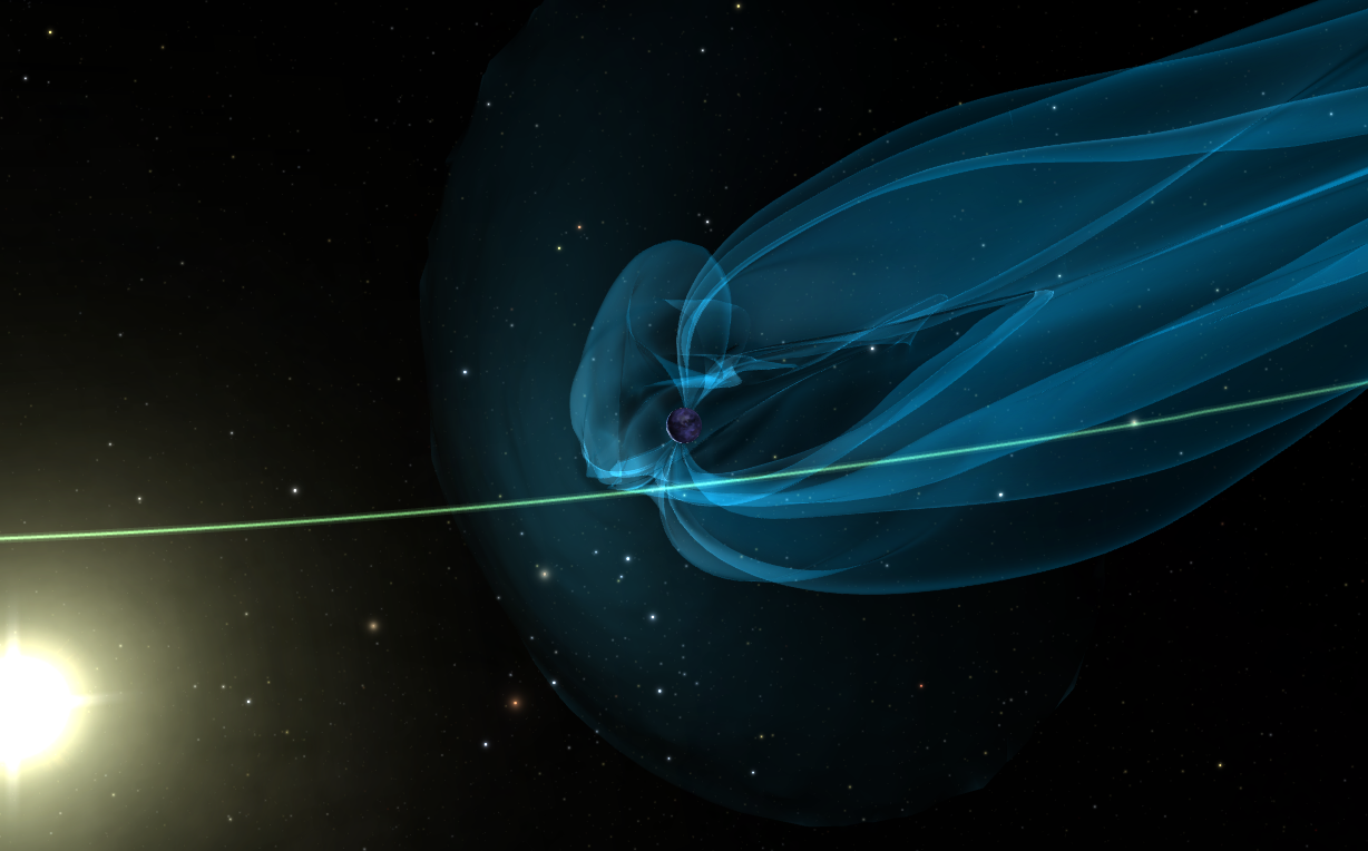
Another aspect of Earth is the fact that we have a magnetic core, which Mars does not have. And this magnetic core actually sets up the magnetosphere of Earth, which is blown back by the solar wind. And we’re protected by this, essentially. It protects our atmosphere. Protects us. So, here, we see the Earth spinning underneath the polar axis. The magnetic axis is slightly off axis of the spin axis. We can see here the magnetosphere. It’s a beautiful object if we could see it. Another thing to note is that it extends out, as you saw just as we approached, I’m sorry I didn’t point it out to you, but it extends out to roughly lunar orbit. To go outside it is extremely dangerous. And the Apollo astronauts knew that when they fly, when they flew to the Moon. We were outside the protective shield of the magnetosphere. And if a major solar event had happened, they would have died.

So as we begin to just bring the Earth back up here to see the diurnal motion once again, focus a bit on the poles. At this point the seasonality, which you’ve just seen demonstrated, is the, the polar wandering in and out into sunlight and back again in the seasons, sets us up for the rest of our discussion tonight. Dr. Ned Gardiner from the National Oceanic and Atmospheric Administration is going to take us through migrations and the human effect. Ned.

Satellite observations

Thanks Carter. The science that you’ve been looking at this evening, was inspired by looking out to the stars, to understand the cycles of the seasons, to understand how moving around a star influences life on Earth. This determines when we should plant crops, when we should harvest them. And tonight we want to look inward and begin imagining for ourselves the new stories about our place on this planet, and the way we’re shaping life on Earth, interacting with a living system and the physical systems on Earth.

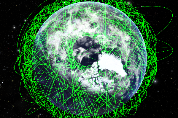
These tracks here are the hundred brightest satellites orbiting our planet. And they’re collecting data for us every second about where we live. Scientific satellites measure reflected radiation from the planet and can tell us important information about the behavior of the physical systems. And what we’re going to explore tonight in about ten quick stories is some of the physical behaviors of our planet and how they drive biological systems on a global scale. This is a unique theater environment where we can begin understanding what thinking globally really is. That’s what we will be doing.

Before turning off the satellites, I want to emphasize that we are looking at data collected from the perspective of our eyes in the sky. And you will notice most of these tracks leave a hole right in the Arctic Ocean. This is just due the orbital mechanics of how to optimize a flight to cover the whole planet. But you will see evidence of our blind spot when we strip away the clouds and bring up a dataset showing ice floating on the Arctic Ocean.

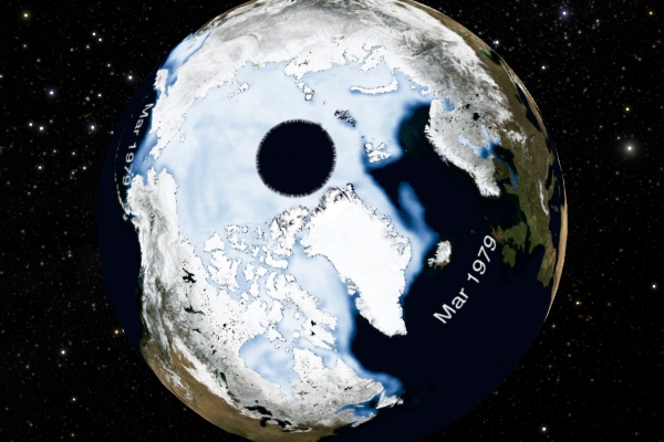
Here’s the data hole I told you about, and that’s simply a fact of our vantage point using satellites not detecting any information there. Now when I started looking at these data about ten years ago, it was reasonable to assume that that hole was covered in ice. But you are going to see that we can no longer make that assumption.

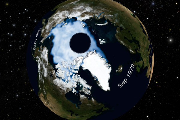
The brighter the white color on these maps, the more ice is present on a patch of sea. And the lighter the color, on the peripheries, the less ice is present. What we’re doing is measuring heat coming off the Arctic Ocean. So where there is open water, we can detect the heat and map a quantity, which is the concentration of ice. Now you will also noticed the month and date changing through 1979, the first year with complete high quality satellite record for Arctic Sea ice in our climate data record. January is not the month of maximum ice. In fact we have to move up to March to see this floating ice reach its maximum. And by September it reaches its minimum.

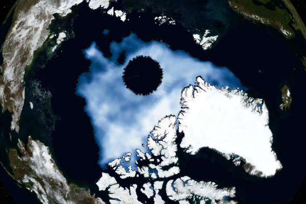
By comparing two data from September 1979 and September 2012, you can see a massive story unfolding. On 16 September 2012, sea ice reached its all-time minimum extent, 20% smaller in area than any other date recorded in the satellite data record over 33 years of data. Compared to September 1979, this reflects a fundamentally different climate system. And when I say fundamentally, I’m not using that lightly. It is widely recognized in the Arctic science community that the Arctic of the 20th century is gone; the Arctic does not behave the same way it did anymore.

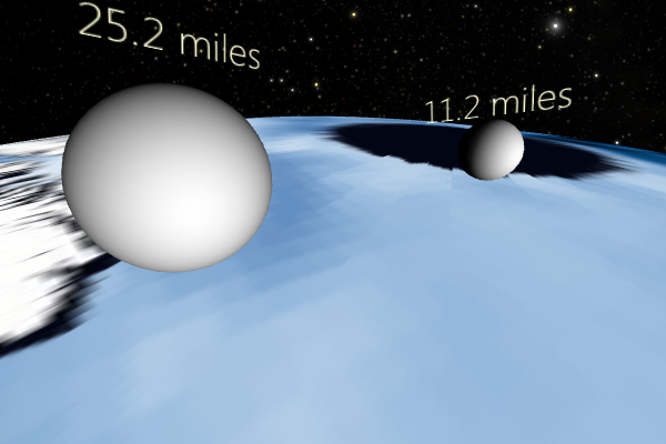
We can visualize this another way by flying closer to Greenland and comparing volumes of ice. Compare this sphere representing the total volume of Arctic sea ice in 1979, correctly proportional to the Earth. That’s the total volume if you made one big ice sphere, from all the ice floating in September 1979. There is an order of magnitude less volume in September 2012.

So is direct evidence of the changing climate. As we pull out, just keep in mind that the physical system of Earth is changing. At the same time, the physical systems of Earth have set expectations by species all over the planet.

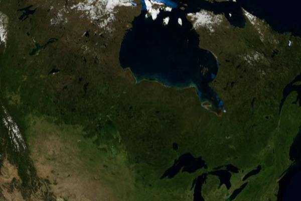
Let’s start simple. Let’s start with the species that harvest sunlight, turn it into energy that we all rely on for food and fiber. And we’ll focus on the Canadian Shield for a moment. We will look at the seasonal cycle of the greening up of plants in the springtime: the flush of the leaves and the production of grasses that happens as the sun reaches high in the sky in the northern hemisphere. And if we advance the months one by one starting at January, we are going to see the retreat of the snowline, and the greening up of the vegetation. This composite image from literally thousands of satellite images shows the response of plants harvesting sunlight, turning it into energy, a very simple concept.

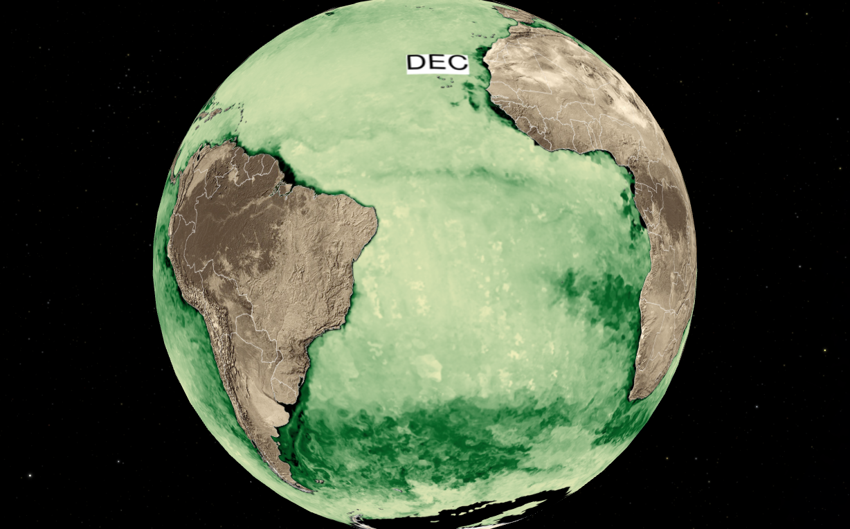
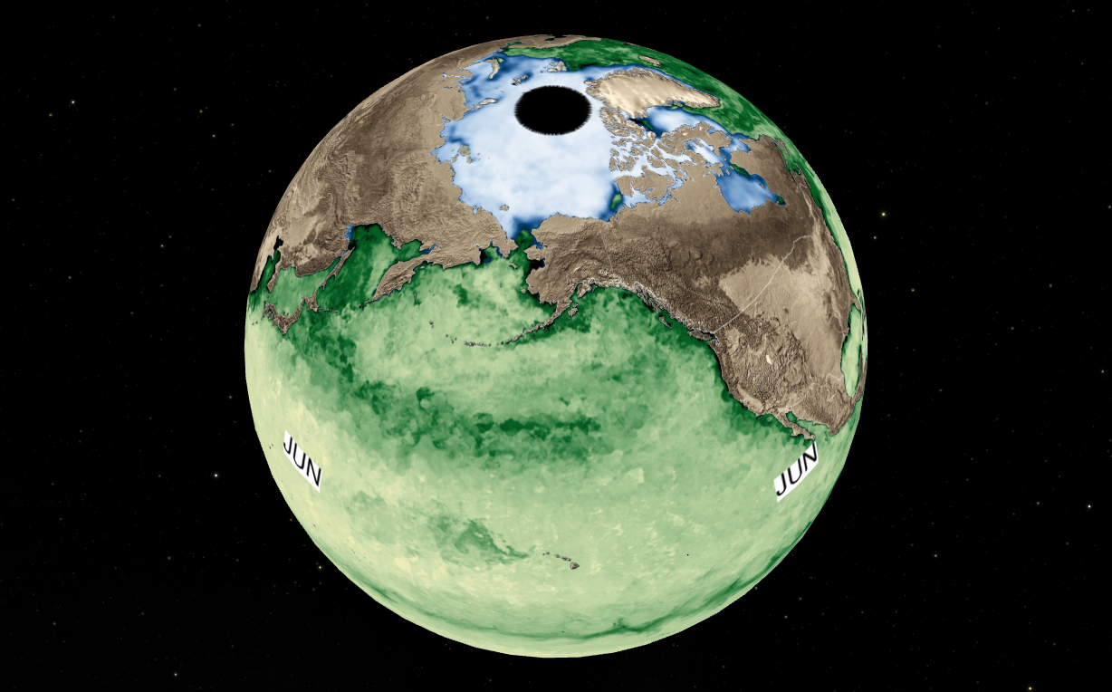
Here’s another way to look at it that maybe you haven’t seen before. The harvesting of sunlight by plants also happens in the global ocean. The ocean is one massive connected ecosystem, and floating in it are microscopic plants called phytoplankton. These are single-cell organisms that use nutrients from the water column, and when there’s available sunlight, they multiply and grow. What you are seeing on is that the darker the color, the more productive (a term ecologists use) the ocean is. This gives more oxygen being produced by plants, more carbohydrates that are being formed by taking up carbon dioxide out of the atmosphere. The lighter colors show the lower productivity areas, where the phytoplankton are not growing as quickly.

In the Arctic in the northern hemisphere winter, a band of black expands; the color represents no data. This is an artifact of the fact that there is not energy being reflected off of the ocean during the wintertime, and hence no reflected radiation to measure. If we go to the southern hemisphere, we will see the same phenomenon during the southern winter.

In January during our northern winter, it is summertime with abundant sunlight in the southern hemisphere. In the south Atlantic Ocean, there is a huge fetch of wind that blows year round, stirring up nutrients from the cold waters of the southern Atlantic. When the Sun strikes these waters, you get massive blooms of productivity. These plants become available to invertebrates to consume. Those invertebrates are available to fishes, some of which we catch and eat and depend on for our protein. Those fishes are also available to larger predators.

As we follow this cycle, we see a massive bloom of phytoplankton along the west coast of North America and all the way across Pacific Ocean. These blooms harvest sunlight, take nutrients and support entire food webs. The Gulf of Alaska is our most productive fishery for the United States. I hope you’ve come to appreciate now that plants in the ocean produce half the oxygen we breathe. They produce a substantial amount of the protein that we consume by feeding food webs, and the fish that we depend on.

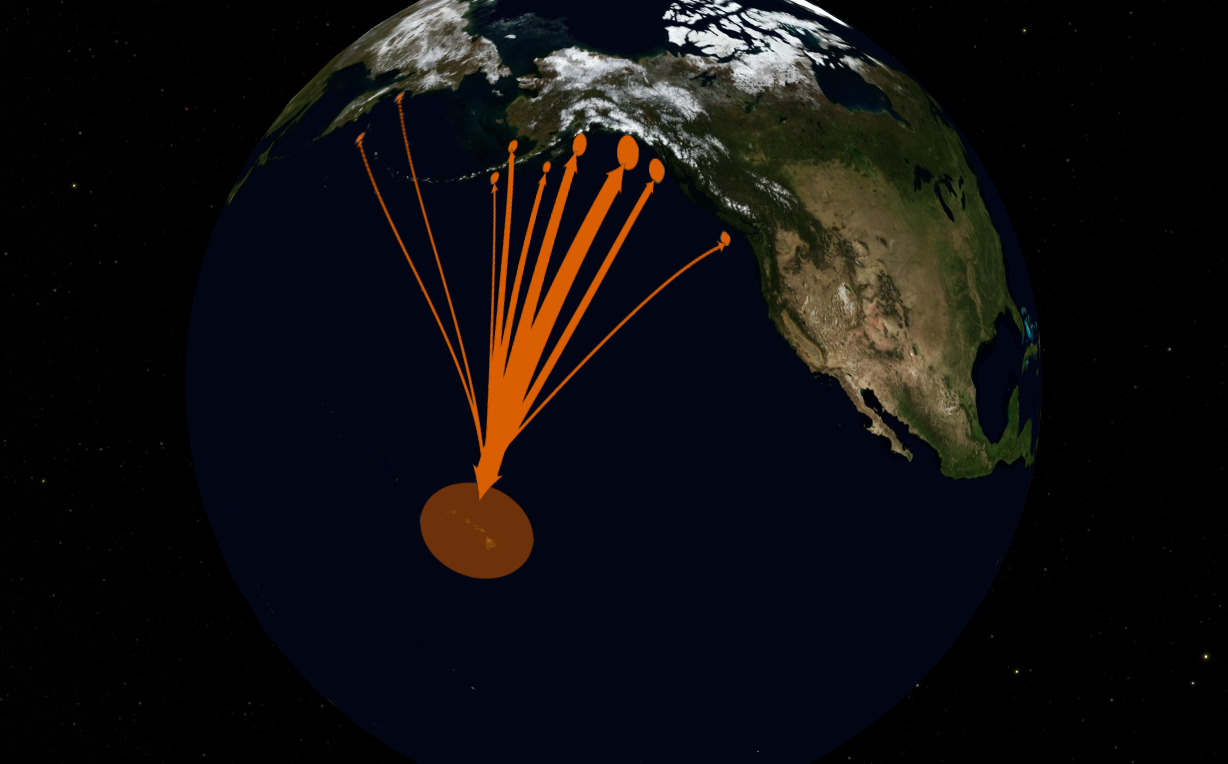
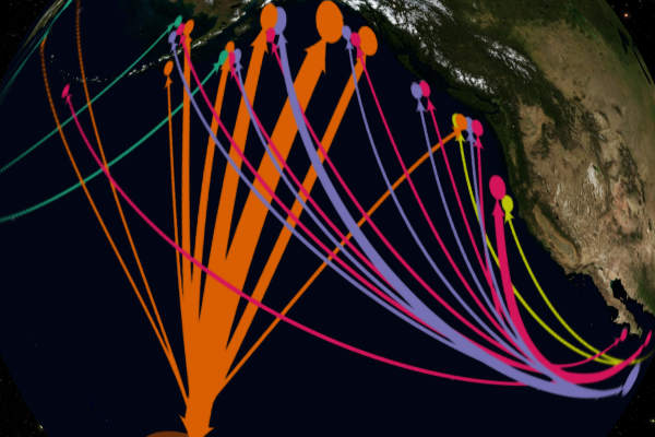
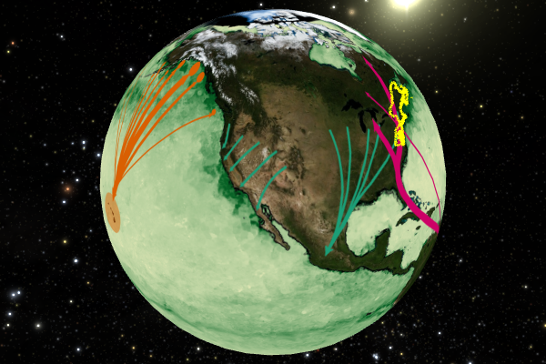
We are not the only species that depends on these huge blooms. We can show you observations of groups of humpback whales that take advantage of the seasonally available food resource in this region, which is such a huge burst of energy available that whales have evolved to take advantage of this. All of these circles here represent different observations by scientists like the Museum of Natural History’s Howard Rosenbaum and his colleagues who identify individual humpback whales by the markings on their flukes, and by the tissue samples they collect. By running genetic analyses on the tissue samples, they can show that whales all across the northern Pacific Ocean come from the same population. They are genetically related. And we can depict that for you with an image that shows how these dispersed organisms all migrate thousands of miles back to Hawaii every year where they breed and calve. This is just one population in the Pacific Ocean. There are other groups of humpback whales that have different calving grounds that also disperse out through the north Pacific to feed in very dispersed areas and then come back together for breeding and calving in Japan, Costa Rica, and Baja California. We can understand entire planetary processes from a macro perspective using satellites, and a micro perspective using genetics. Those are just two ways that we are learning, even today, about how animals are synced with the seasonal patterns on our planet.

Marine protected areas - series along the coast. California is a leader in this effort. This is a community effort - scientists, diver, fisher people, users, etc…

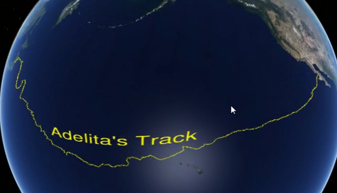
What really distinguishes migrations among all species is the drive, the determination of individuals and in whole populations of species to migrate in a direction to take advantage of a resource. And there’s a really wonderful story about this kind of determination in the story of Adelita who was a loggerhead turtle that a fisherman caught near Baja California, and a researcher from the California Academy of Sciences in 1996 decided to help this fisherman, because this loggerhead turtle had outgrown its captive habitat. So they glued a radio-transmitter on the shell of this turtle that sent signals up to satellites so we could see where this turtle would go. And boy, did Adelita go. She went 6000 miles across the Pacific Ocean, all the way to Japan.

Site Fidelity

Remember that this was a captive organism, and as a result changed people’s thinking about sea turtles in a fundamental way. It turns out that all sea turtles share this determination. Here we see leatherback sea turtle tracks. These leatherbacks nest all in the western Pacific, but will return to the beach where they were born. The females will return to the beach where they were born in order to lay eggs. And that’s what they’re doing in this eastern part of their range. They migrate all the way across the Pacific Ocean to feed on jellyfish off the coast of California.

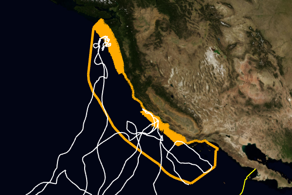
Species that move this far are clearly subject to a number of influences over such a large area. One of the things that ocean conservationists are focusing on is the importance of zones where we can exclude fishing activity, and limit recreation to non-invasive types of activities. And that’s what you see here depicted in the network of marine reserves off the western coast of North America. We can also show a whole zone where management activities are focused on helping entire food webs and entire ecosystems (groups of organisms and their habitat), to function naturally and be resilient.

Resilience is a very important idea. What it means is that if a change perturbs a system, that system can respond and continue to function in a normal way after some period of stabilization. So building resilience is one of the key ideas of building marine reserves as well as reserves on land.

Let’s move to land. I promised I was going to give you a series of somewhat unrelated stories, but the point here is to focus on the idea of migration and the connectedness of different ecosystems along the journey of a species that depends on the resources in different parts of the planet.

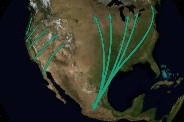
Monarch butterflies are a wonderful example. They spend their winters in central Mexico, in very localized fir forests. And because they are so vulnerable in this one area, conservationists have been very effective in protecting them by setting aside and managing lands, preventing logging in this critical habitat. What is amazing about this organism is that when it sets off north to take advantage of the spring and summer flushes of milkweed in Texas, in the central United States and in the upper Midwest, they will reproduce along the way. Literally four generations later, whole groups of monarchs arrive from a habitat thousands of miles away without any possibility of direct memory of this same habitat. But they make this directional journey, and return again every year. So it’s quite a wonderful mystery that biologists are looking into it.

Remember the magnetosphere that Carter put up. It’s thought that insects and birds and, and, perhaps mammals as well use the magnetic field of Earth as well as terrain cues to navigate, to understand where they are in space.

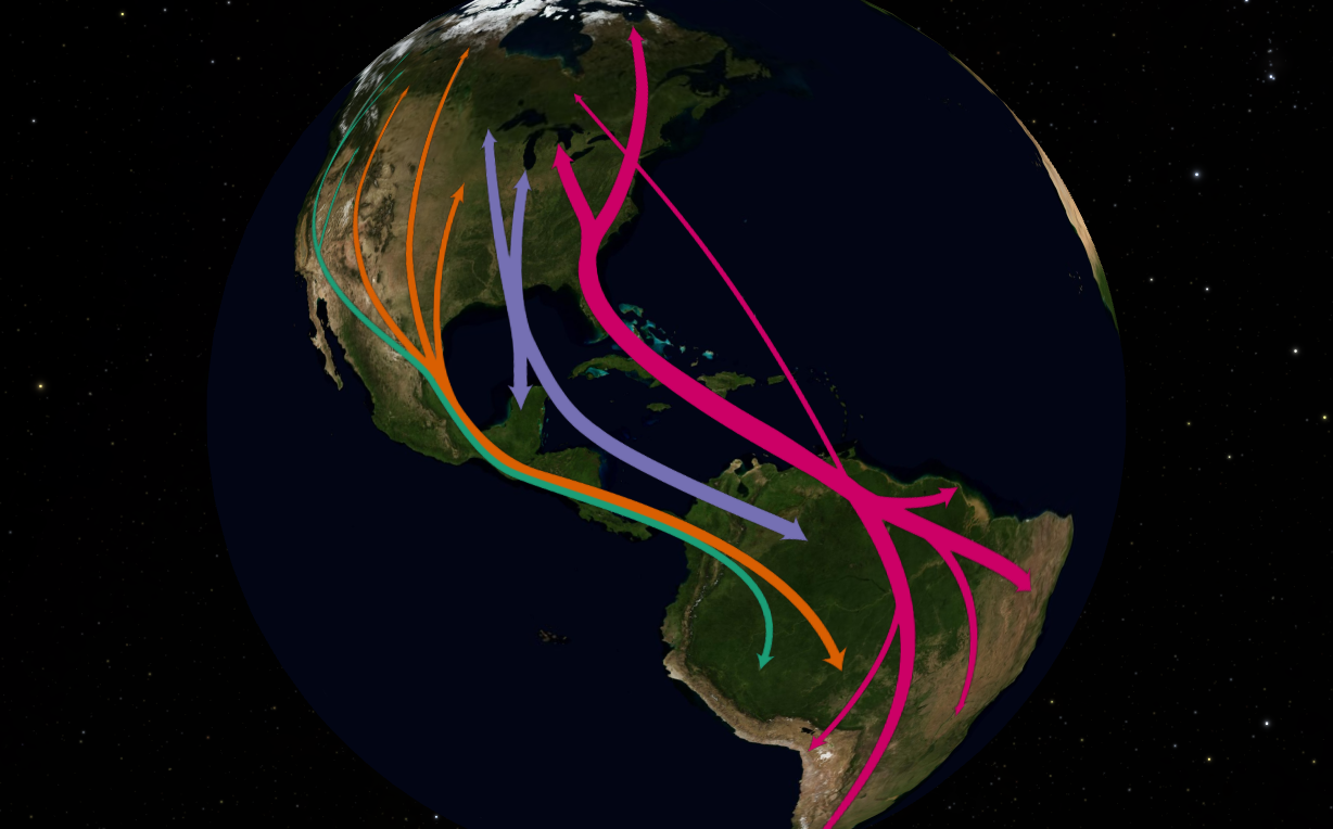
Let’s think about birds next. Many of you probably know that there are some distinct highways of life, pathways where birds fly. There’s the Pacific flyway, the Central flyway, the Mississippi, and the Great Atlantic flyway. If you (here in Manhattan) go to Central Park in spring or fall, you might observe one or more of over 230 species of bird that fly through, depend on, and use your treasure in your backyard that Frederick Law Olmsted designed for your enjoyment. And that patch of wild earth is essential for birds stopping over on a much longer journey that connects our continent with South America and with the Caribbean. And it indeed connects our country with nations all along, throughout this hemisphere. This flyway has inspired the imagination of conservationists to think about how we can cooperate internationally to understand what kinds of habitat changes might be happening thousands of miles away that affect the birds that we depend on, and which we care about in our backyard.

Here you see, for example, the Atlantic flyway reaching all the way to Patagonia, to the southern tip of South America. There literally are birds that fly from pole to pole every year.

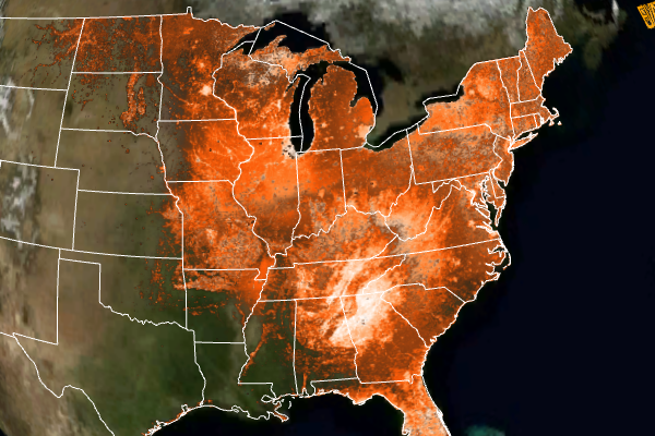
We’re going to go back to North America and show you some of the complexity of an actual migration path of the Blackpoll Warbler, which is a small songbird which has the unfortunate distinction of being the fastest declining songbird in North America. Between 1980 and 2007, this bird was declining at 10% a year, so that today the population is some 10% of its historic numbers. This map is a composite map; what we see is a whole year’s worth of data combined together.

When we start the animation, look for the month indicator in the Atlantic Ocean to the east of Maine.

People who are passionate about birds go out and observe what species they hear and see, and they submit their observations to the Cornell Ornithology Laboratory. If people spotted only a few Blackpoll Warblers, you would see patches of very faint orange dots. More and more observations get depicted in this map by brighter orange, then white colors. The intensity of the color maps represents the probability of seeing a bird. I want to emphasize that this is a massive human enterprise involving literally 100,000s of locations and people.

Now we’re going to progress through every month of the year and show you the flight path of Blackpoll Warblers as they come from the Amazon in South America as well as the Caribbean up through North America on their journey north to take advantage of the flush of insects during the spring and summer. Every time the month flashes, a new image is loading. These maps only cover the United States, and so we are not seeing their entire range. If we had complete maps, they would show where these birds are in Canada. When it’s wintertime here in the northern hemisphere, there is no data. But in mid-April, we are going to see the emergence of the first observations of Blackpoll Warblers, first in Florida. And watch as they move through.

We see the movement and the directionality of movement along the eastern half of North America up through New England. At the end of summer and fall, they come back, congregating on the east coast of North America before taking a massive, non-stop direct flight, the Blackpoll Warblers head south to the Caribbean and to South America. The reason they can do that is they have taken advantage of the flush of insects during our summertime, and have fattened up. The increase of vegetation we saw before, responding to sunlight, is associated with massive population increases of insects that Blackpoll Warbler feeds upon.

During its northward journey, Blackpoll Warbler stop in habitats all through eastern North America. While they are not here for very long, they are subject to any chemicals we have in our backyards; or if our buildings aren’t bird-safe, they might have an accident against a window; or they can meet their demise in other ways. Which is why conservationists are concerned about the complete range of a species like this, that occupies whole hemispheres during its journey, and during its various life-stages.

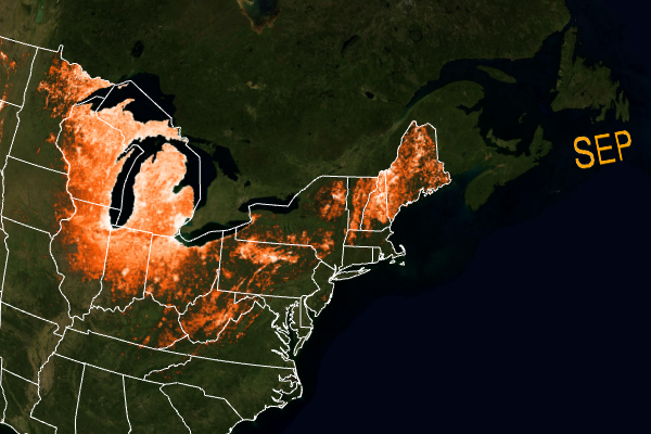
And, let’s just bring up one image showing the June distribution of Blackpoll Warbler in northern New England, with the state lines on for reference. Throughout the summer you might be able to observe a Blackpoll Warbler nesting in the high elevation spruce and fir forests of northern Maine. This elevation is associated with these forest types at this latitude, where the climate is colder, and more suitable for the Blackpoll Warbler.

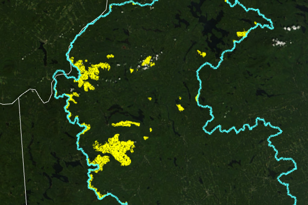
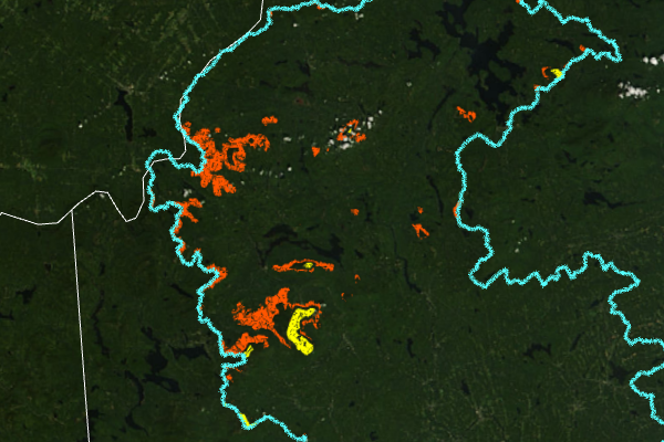
Let’s bring up the Kennebec River watershed where University of Massachusetts researchers are using computer modeling and observations of the natural history of Blackpoll Warbler to understand where it nests today and where it’s likely to nest in the future. These yellow areas represent the current optimal area for Blackpoll Warbler, and this includes the climate and habitat preferences for today’s population. They need these spruce trees to forage for the insects that they eat, and they need cool conditions for their metabolism. But in the future, we know that climate is changing, and this range is going to contract. And here you can see the orange areas as zones of contraction for this species in the year 2030. That’s not very far away. But by 2080 this Maine sub-population of Blackpoll Warblers is not going to have very many optimal areas where it can nest. The red is likely to show an underestimate of the shrinkage, because this model averages together a whole series of scenarios all of which we are exceeding right now. The surface imagery also conveniently shows a non-climate driver of threats to the species, which is deforestation through logging activities. You can see it very clearly in satellite data. (One of the great applications of satellite data in conservation biology is to be able to detect changes in land use.)

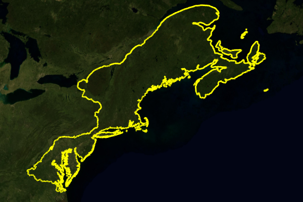
By incorporating our understanding of land use and climate and habitat preference, conservation biologists today are able to synthesize and take a big-picture perspective on a single species that represent conditions important for other species. We call this a representative species, and in this case Blackpoll Warbler represents the high elevation fir forest type. But we can also think about whole suites of species and integrate this information to think about landscape-scale conservation. And that’s really the mission of the North Atlantic Landscape Conservation Cooperative, the boundary of which is drawn on here. Now, notice the state lines all have rigid north-south directionality, although they might follow a river here and there. But the boundary of the North Atlantic Landscape Conservation Cooperative follows an ecologically relevant association of geology, rivers, and vegetation types.

The North Atlantic Landscape Conservation Cooperative is a, really a pioneering effort—by conservation biologists, government agencies, researchers such as those at the University of Massachusetts whose data that we were just looking at, tribes, governments and non-governmental organizations—to think about multiple kinds of stresses in our local ecosystems and make decisions today that really matter for the ecosystems that our grandchildren will inherit. One great example of that is looking at the resilience of whole landscapes. We can take a species approach, but we can also look at whole landscapes, the geology, and the vegetation.

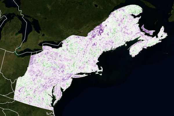
Let’s look at resilience throughout this North Atlantic region. This is a map made by the Nature Conservancy that really simplifies a very complex idea into just something very easy to look at. The large patches—such as in the Adirondacks, or in northern Newfoundland, or the Pine Barrens of New Jersey—are the critical intact areas that are likely to be the most resilient to a changing climate and changing land use. We can look at the inverse which are the less resilient areas. Those areas are where we need to take special measures in design. The opportunity is to design the way we live to facilitate other species such as the green building codes now for Manhattan, like the New York Times headquarters is LEED certified to protect birds, so that they don’t die against the windows of the buildings. It’s a pretty basic preventative measure we can take, but we really do have opportunities.

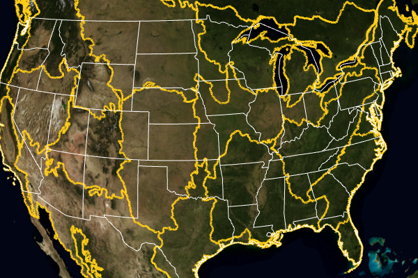
And so I just want to leave you with this idea that the Landscape Conservation Cooperatives are giving us sort of an integrated view that allows us to make better decisions. There are twenty-two such cooperatives throughout the country. You can see just in the satellite data why it makes sense to draw the boundaries the way we do. You can see the coastal plain from the Mississippi River, the upper Missouri River, the Colorado Front Range, the Great Plains. You can see how nature’s boundaries might be drawn, based on mountains, rivers, and vegetation types. That is really the organizing principle of the Landscape Conservation Cooperatives, and the reason why we ecologists think differently than political boundaries. And indeed, these boundaries span international boundaries.

We have just taken a journey that included Earth cycles and the natural variation of sea ice. The fundamental lesson from all of these journeys—looking at sea ice, whale migrations, butterflies, and flyways, Blackpoll warbler—is that Earth is changing in some fundamental ways and we are observing it in real time. We do not have the words yet to describe what we are seeing. For example, literally Arctic peoples cannot describe the birds that they see now in the springtime because they are new to that part of the world due to a changing climate. I had someone tell me that he saw with his own eyes bears in the Arctic preying on and trapping whales, because they no longer have access across the pack ice to walruses and seals that they depend on to eat. We literally have a changing planet that is difficult for us to describe.

But tonight, we have taken a journey. It is a very important new idea for humanity which is to develop an understanding, visually, of what is happening on our planet, so we can have more sophisticated conversations than just what you believe and do not believe. This is about what’s happening. Observations on our planet that inform us in all walks of life about what we can do. And, so, tonight’s presentation really was just a first step. I hope in helping you all have conversations in your daily life informed by a new mental image of what’s happening on our planet.