
Storyboard · WvN11

Forests, Beetles, and the Cycles of Life

Vast stands of coniferous forest are an essential part of the ecology, economy, and character of western North America. Recent dramatic changes, such as forest mortality from insect outbreaks and increased fire activity, are occurring across huge areas of western forests. This Worldviews Network production offers an immersive journey into the past, present and future of our forests. Travel through space and time to understand the connections between local forest ecosystems, global forest biomes, and our cosmic neighborhood to explore how and where the pine beetles are changing the Colorado landscapes, how these infestations arose, and their impacts on forests of western North America.

Premiered
June 4, 2013
Venue
Gates Planetarium, Denver Museum of Nature & Science
Scenes
41
Last revised
February 3, 2014

Web version · Original script and storyboard (Google Doc) »

01

Cosmic: Conditions for Life

3 scenes
Scene 1.1, frame 1
Scene 1.1

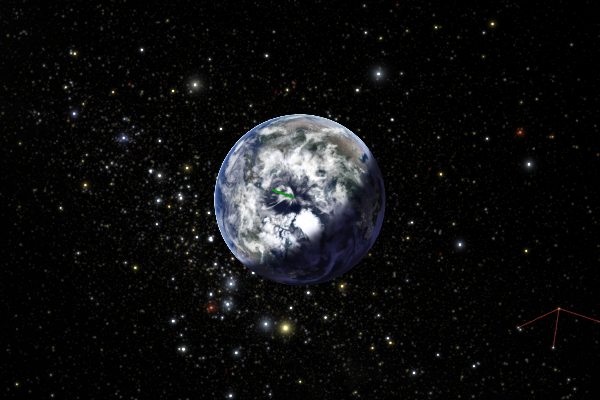
We’ve started out looking at the Earth from space. You might wonder why is it that we choose to talk about the Earth from space. It’s because the same instrumentation that we put on satellites to observe the stars and the rest of the heavens can also be turned on downwards to view our home planet.

Magnetosphere

Now, one other thing that we’ve learned since the space age is the fact that the rest of the cosmos has impact on not only Earth but on life on the Earth as well. And so here we are seeing a visualization of the Earth’s magnetic field, its magnetosphere. We’ve known for a long time that the Earth has a magnetic field given the fact that navigators have used compasses for many centuries. But it was only after the dawn of the space age that we realized that this magnetic field protects the Earth’s atmosphere from the solar wind, preventing it from being stripped. And it also protects life from cosmic radiation.

Uniview cues
Browser Control (1a. NPP tab)
Jump to START Bookmark button
Magnetosphere Toggle button
Geoscope Layerset:
Load wvn11_dmns_1a_FINAL.layerset
Sources

Earth’s magnetosphere and bow shock is based on model from Charles Goodrich and group (Boston University) of effects from the “Halloween Solar Storms of 2003.” For more information about the storm, see this USGS website, and the 2004 NOAA report Service Assessment: Intense Space Weather Storms october 19 - November 07, 2003 (PDF). Also see the links here and here.

Created by the American Museum of Natural History and SCISS/AB.
USGS website

PDF

here

here

Scene 1.2, frame 1
Scene 1.2

Habitable Zone

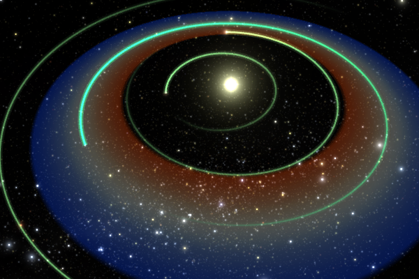
Now we will fly above the plane of the solar system . We see Mars, Venus and Earth. The visualization toggled on is the habitable zone. This colorful region shows where in the solar system liquid water can exist on surfaces of rocky planets. We think that Mars and Venus actually had very similar conditions to Earth early in the solar system. But because they lay just on the edges of the habitable zone, and because of other different factors, both of them have dried out and have either become extremely hot or extremely cold. And it’s only on Earth do we have a place where life is abundant.

Uniview cues
Browser Control (1a. NPP tab)
Jump to HZ Bookmark button
Habitable Zone Toggle button
Sources

Habitable zone marker for the Solar System, created by California Academy of Sciences and SCISS/AB.
Scene 1.3, frame 1Scene 1.3, frame 2Scene 1.3, frame 3
Scene 1.3

Seasons

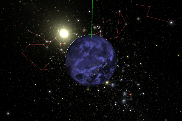
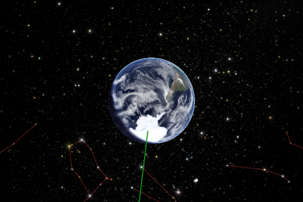
One other aspect I want to talk about as it relates to life here on Earth is the fact of the seasons. The simulation has been set to the June 21st solstice. The poles of the Earth are visible so you can see where the north and south poles are. We start moving forward through time going one day per second. You can see that on the June solstice, the North Pole is completely in sunlight and, in fact, the northern hemisphere receives more sunshine than the southern hemisphere.

And this is the main contributing factor to our experience of the seasons on the Earth. It’s not due to the fact that Earth travels slightly closer and slightly further from the Sun. That is a factor but it’s negligible compared to the tilt of the Earth. And as we keep moving forward through time, as the Earth continues in its orbit, the relative tilt is going to bring us to the fall. At the September equinox, both the northern and southern hemispheres are receiving equal amounts of light; we actually get twelve hours of day and night for the entire Earth.

And as we keep moving through time we will find ourselves at the December solstice. The sunlight patterns have reversed themselves; we are seeing Antarctica in full light, and the Arctic in complete darkness for the entire day. This cycle not only affects the Earth but also anything on its surface.

And it’s the Earth’s relationship to this cosmic environment that produces seasonal cycles that support life.

These seasons have been a persistent feature of our planet since the formation of a biosphere almost 4 billion years ago. And as we will see, life on Earth has been shaped by these seasonal cycles.

Uniview cues
Browser Control (1a. NPP tab)
Jump to JUNE Solstice Bookmark button
Poles Toggle button
Lat-Lon Toggle button
Ecliptic Toggle button
Uniview Controls:
Demo and show seasons through the year by setting simulation time velocity to 1 day/sec, setting time in motion, and scrubbing forward to equinoxes and solstices.
At each equinox and solstice, can stop and show the different mix of lighting and shadow on the northern and southern hemispheres.
02

Global: Satellites

1 scene
Scene 2.1, frame 1Scene 2.1, frame 2
Scene 2.1

Satellite observations

In the past 50 years, we’ve been gaining new insights into these cycles through Earth-observing satellites, which we like to call our eyes in the sky.

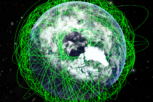
And we’ll show you many datasets tonight derived from these satellites that instead of viewing space, are viewing our home planet. These are the hundred brightest satellites that are orbiting Earth right now. These satellites allow us to study otherwise invisible patterns and interactions of Earth, air, fire, and water across the planet.

And as we fly around over the North Pole you can see a data hole. The satellites orbit in a way to intentionally miss going exactly over the North Pole, because it makes them a bit more efficient mapping the rest of the Earth. And in some of the datasets that you will be seeing, you will actually see a hole like this.

Uniview cues
Browser Control (1a. NPP tab)
Satellites: 100 Brightest Toggle button
Satellites: Orbit Type Toggle button
Geoscope Layerset:
Load wvn11_dmns_1a_FINAL.layerset
Uniview Controls:
Start time moving (at least 1 min/sec) and fly around the Earth. Toggle satellite orbits between trails and lines.
Sources

100 brightest satellites orbiting Earth based on Two-Line Element sets from NORAD, available, e.g., here.

Prepared by SCISS/AB.
here

03

Global: Seasonal Changes

12 scenes
Scene 3.10, frame 1
Scene 3.10

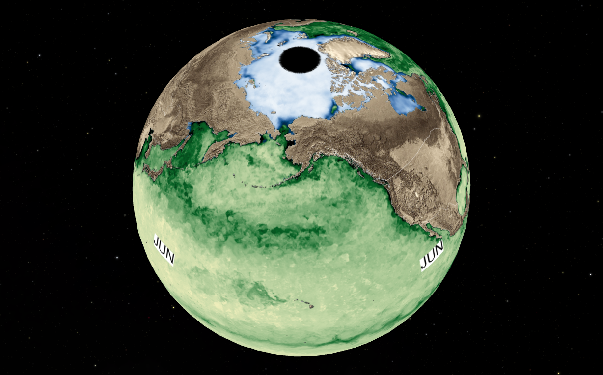
Net Primary Productivity in Oceans

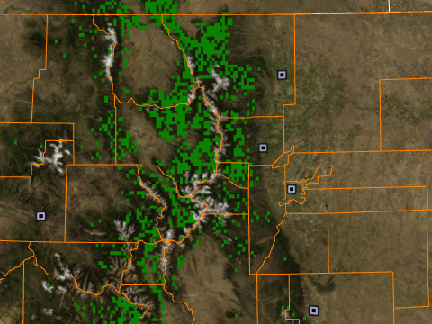
We are going to observe one of the most essential of all life’s processes: The response of life to Earth’s annual orbit around the Sun. Here on the ocean’s surface which covers almost three-quarters of the planet, we are watching massive blooms of microscopic floating plant life called plankton. The dark green are blooms of plankton responding to the Earth’s, responding to solar radiation that’s coming in cycles we just observed from the seasons.
During winter, that energy’s weak. It limits growth. But now here we are in summer and we see huge bursts of plant life that are visible as dark green blossoms in the ocean’s northern regions. We are literally witnessing the process of photosynthesis in the oceans, which combine solar energy, nutrients, carbon dioxide to create life and produce oxygen.

With each emerging band of dark green, we are actually watching the formation of the base of the marine food chain. With the seasons of ocean photosynthesis during this sequence, we can imagine the Earth is breathing. The biosphere is inhaling in the summer and exhaling in the winter. A long annual, cyclical breath.

Uniview cues
Browser Control (1a. NPP tab)
Load Layerset #1a button
Weekly NPP/Monthly Arctic Sea Ice:
Reset Cycling button
Cycle Once button
Continuous Cycle buttons
June NPP button
Dec NPP button
Geoscope Layerset:
Load wvn11_dmns_1a_FINAL.layerset
Uniview Controls:
Slow pan focused on the Pacific Ocean.
While over North and South America: review patterns, once over the rotation of each hemisphere throughout a year. See differential pattern of biomass in the ocean hemispheres.
Scene 3.20, frame 1
Scene 3.20

Cryosphere and Greenup

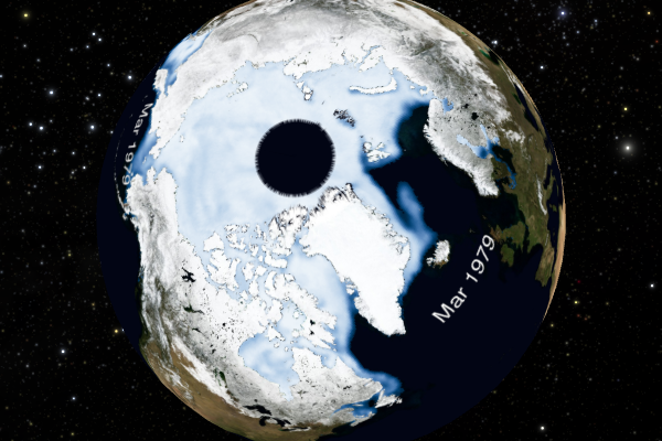
We can also see this cycle on the land, and it mirrors much of what we saw in the ocean. We will watch photosynthesis on land in the northern hemisphere. We’ll see that in the northern reaches at the beginning of the year snow and ice cover the ground during the cold, short days of winter.

Those cold, short days of winter prevent a lot of photosynthesis. But as spring arrives, the snow retreats and it sets the stage for a burst of life that arrives with the summer. We are watching the greening of Eurasia. And we will go back and play it again and watch the greening of North America.

This summertime greening of the land in the northern hemisphere sweeps across the grasslands and forests. And then the cycle repeats itself when the shorter days of fall arrive. Plant growth declines, and eventually the snow comes back to cover the area.

Uniview cues
Browser Control: (1b. BMNG+Sea tab)
Load Layerset #1b button
Monthly BMNG/1979 Arctic Sea Ice:
Reset Cycling button
Cycle Once button
Continuous Cycle buttons
16 Sep 2012 button
Geoscope Layerset:
Load wvn11_dmns_1b_FINAL.layerset
Sources

Arctic Sea Ice and Blue Marble Next Generation with monthly labels. Visualization by Hunter Allen. Data from National Snow and Ice Data Center (NSIDC; http://nsidc.org/). Compiled by Ned Gardiner.

bmng_ice_197901.kmz

bmng_ice_197902.kmz

bmng_ice_197903.kmz

bmng_ice_197904.kmz

bmng_ice_197905.kmz

bmng_ice_197906.kmz

bmng_ice_197907.kmz

bmng_ice_197908.kmz

bmng_ice_197909.kmz

bmng_ice_197910.kmz

bmng_ice_197911.kmz

bmng_ice_197912.kmz

bmng_ice_20120916.kmz

Blue Marble Next Generation

http://nsidc.org/

Scene 3.31, frame 1
Scene 3.31

Global: Keeling Curve

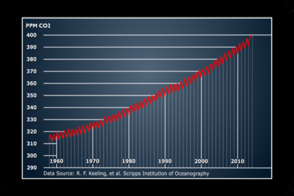
These seasonal cycles of life in the ocean and on land can actually be seen in the composition of Earth’s atmosphere. You see a graph of the measurement of carbon dioxide in the atmosphere over the last fifty years. And perhaps the most startling aspect of this curve is the oscillation. Every year the annual cycle of photosynthesis in the northern hemisphere registers. The down part is the inhalation of carbon dioxide with the burst of northern hemisphere plant productivity, and then the release of that process accumulates carbon dioxide in the atmosphere in the fall and winter.

We literally are seeing the cycle of life registered in the composition of carbon dioxide in our atmosphere. The other salient feature of this curve is that it’s only going in one direction. This curve doesn’t level off. It just keeps going up and up. And on May 9th, 2013, we crossed the threshold for the first time ever: 400 parts per million of CO2 were registered in our atmosphere.

But what this oscillation shows us is direct evidence that plants can help us absorb carbon pollution. They’re part of the solution for how we will manage the carbon concentrations of the future. These seasonal cycles also drive other patterns of life on Earth: patterns of temperature, precipitation, and fire.

Uniview cues
Browser Control: (3b. Panos & Slides tab)
Keeling Curve: 1958-2013 button
ALL SLIDES OFF button to turn off
Sources

Visual by Hunter Allen at NOAA. Data from NOAA’s Mauna Loa Observatory (http://www.esrl.noaa.gov/gmd/obop/mlo/). Compiled by Ned Gardiner.

wvn11.ad_keeling_curve_v7.jpg

http://www.esrl.noaa.gov/gmd/obop/mlo/

Scene 3.41, frame 1
Scene 3.41

Average Temperature

Global: Climate

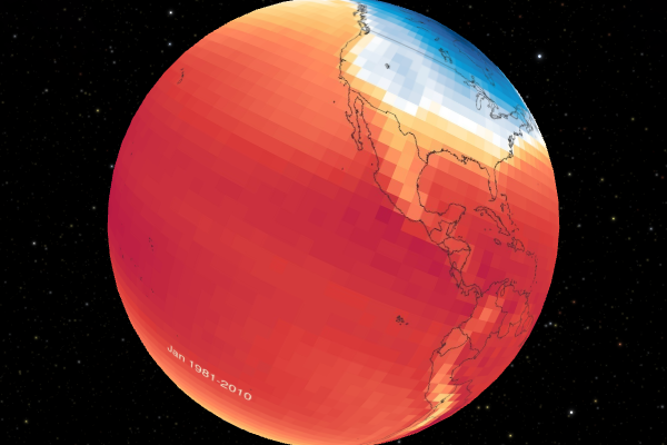
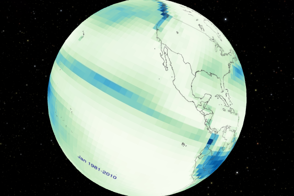
Now you see global temperature patterns from pole to pole going month by month across the planet. They are averaged over the last 30 years where the dark blue is the cold and the dark red is the warm. Month by month the effect of latitude and time of year combine to create patterns. The dark blue moves towards the equator in winter and it retreats in the summer reflecting the strength of the Sun’s energy through the seasons.

That steady red band around the equator stays the same year around. The pattern shows very little fluctuation around the equatorial belt. Of course, these are averages, and so much variability, like a cold snap or heat wave, lies behind these values. The crazy weather that we all talk about over the morning coffee we are averaging and smoothing out here. But we are observing the general patterns of annual temperature across the Earth.

(Another pattern is continentality, or distance to water. This is the moderating effect of being near the coast and large water bodies. The deep interior of a continent fluctuates more in temperature, while the coasts fluctuate less.)

Uniview cues
Browser Control: (1c. Precip + Temp tab)
Load Layerset #1c button
Average Global Temperature:
Reset Cycling button
Cycle Once button
Continuous Cycle buttons
Average Global Temperature Legend Toggle button
Geoscope Layerset:
Load wvn11_dmns_1c_FINAL.layerset
Scene 3.42, frame 1
Scene 3.42

Average Precipitation

The seasons also drive patterns of precipitation. And just like temperature, latitude and time of year influence where rain and snowfall across the globe. The darker blue colors are the highest degree of precipitation and the white colors are where no rain is falling. These are again daily values averaged over a month.

We can see the summer monsoon in Asia. We can see the equatorial belt. You will see a belt of blue move up and down across the equator. You will also see vast parts of the planet where not much rain is falling at all. These are generally the desert regions. Here is the Sahara, and the annual cycle of rain that moves up and down the belt just below the Sahara. Coming into view is the Amazon rain forest, a forest so dense it actually creates a lot of its own rain.

Uniview cues
Browser Control: (1c. Precip + Temp tab)
Load Layerset #1c button
Average Precipitation Temperature:
Reset Cycling button
Cycle Once button
Continuous Cycle buttons
Average Global Precipitation Legend Toggle button
Geoscope Layerset:
Load wvn11_dmns_1c_FINAL.layerset
Uniview Controls:
Circle the globe to point out monsoons in Asia and rain band in sub-Saharan Africa.
Scene 3.51, frame 1
Scene 3.51

Global: Fires

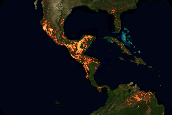
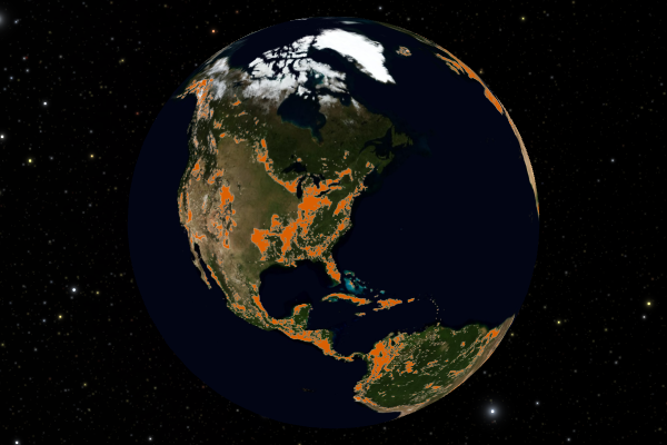
Seasonality of precipitation is intimately tied to cycles of fire on the planet. Now you see satellite data that in near real time registers the occurrence of fire. We are going to see a dataset that goes every month through the last year all the way through March 2013. These images are registering in each pixel the fires that are observed.

And as we go month through month, we will see an astonishing amount of this planet is burning at any given time. That the seasons of precipitation influence when the fire seasons are. That during the dry season it’s also the fire season. And from the sheer extent of fire that we are seeing, it’s clear that life on Earth must be fire adapted as fire is a fact of life on Earth.

Uniview cues
Browser Control: (2.Fires + Forests tab)
Load Layerset #2 button
Active Fires:
Reset Cycling button
Continuous Cycle buttons
Jan, Feb, Mar, Apr, May, Jun, Jul, Aug, Sep, Oct, Nov, Dec buttons
ALL OFF button
Average Global Precipitation Legend Toggle button
Geoscope Layerset:
Load wvn11_dmns_2_FINAL.layerset
Uniview Controls:
Circle the globe to point out fires on different continents, but at the end, fly back to western North America.
Sources

Active Fires (1 Month - Terra/MODIS)

http://neo.sci.gsfc.nasa.gov/view.php?datasetId=MOD14A1_M_FIRE

The red, orange, and yellow pixels on these maps show the locations where the MODIS instrument on the Terra satellite detects actively burning fires. Don't be fooled by sizes of some of the bright splotches on these maps. The colors represent a count of the number of fires observed within a 1,000 square kilometer area. White pixels show the high end of the count — as many as 100 fires in a 1,000 square kilometer area per day. Yellow pixels show as many as 10 fires, orange shows as many as 5 fires, and red areas as few as 1 fire in a 1,000 square kilometer area per day.

modis14_active1month_fire_2012-05-01.kmz

modis14_active1month_fire_2012-06-01.kmz

modis14_active1month_fire_2012-08-01.kmz

modis14_active1month_fire_2012-09-01.kmz

modis14_active1month_fire_2012-11-01.kmz

modis14_active1month_fire_2012-12-01.kmz

modis14_active1month_fire_2013-01-01.kmz

modis14_active1month_fire_2013-02-01.kmz

modis14_active1month_fire_2013-03-01.kmz

modis14_active1month_fire_2013-04-01.kmz

modis14_active1month_fire_2013-09-01.kmz

view.php

Scene 3.55, frame 1
Scene 3.55

RMNP Fires

Patterns of fire and patterns of life have co-evolved, including in our own forested landscape. Now we will take a detour to our own forested landscape and look at the fire history of Rocky Mountain National Park. We will zoom from the global into the continental and down to the very local level to understand that recent fires are actually an ancient phenomenon.

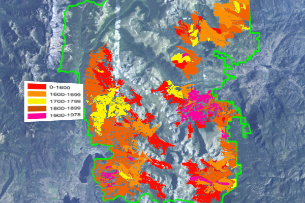
This is the boundary of Rocky Mountain National Park. Dr. Jason Sibold, a researcher from Colorado State University, has reconstructed 2000 years of fire history in the Park by looking at fire scars and soil samples throughout the Park.

Each of the colored shapes in the southern part of the park represents about a hundred years of fire. These layers go from 1 to 1600 AD, with the different colors representing centuries where fires occurred that were intense enough to actually transition the species composition of these forests. So it’s clear there is a 2000 year history of fire in Rocky Mountain National Park. And that, century after century, parts of the park have burned enough to change the species composition. The forests that we recreate in today are actually influenced by the legacy of fires in the past.

Uniview cues
Browser Control: (2.Fires + Forests tab)
Load Layerset #2 button
RMNP Historical Fires Toggle button
Optional Borders:
US States Toggle button
CO Counties Toggle button
Geoscope Layerset:
Load wvn11_dmns_2_FINAL.layerset
Sources

Data contributed by Ron Thomas at Rocky Mountain National Park and compiled by Cynthia Powell.

Jason S. Sibold, Thomas T. Veblen, and Mauro E. González, 2006, “Spatial and temporal variation in historic fire regimes in subalpine forests across the Colorado Front Range in Rocky Mountain National Park, Colorado, USA,” Journal of Biogeography, 33(4), pp. 631–647.

RMNP_outline.kmz

recent_fires_near_RMNP.kmz

wvn11_0000_1600_v2.kmz

wvn11_1600_1699_v2.kmz

wvn11_1700_1799_v2.kmz

wvn11_1800_1899_v2.kmz

wvn11_1900_1978_v2.kmz

wvn11_RMNP_fire_history.kmz

wvn11.cf_RMNP_fire_legend.jpg

Scene 3.61, frame 1Scene 3.61, frame 2Scene 3.61, frame 3
Scene 3.61

Global: Forest Biomes of Today

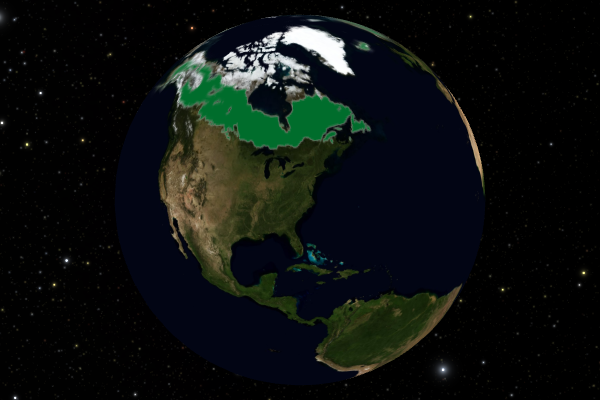
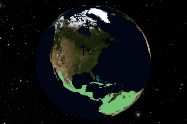
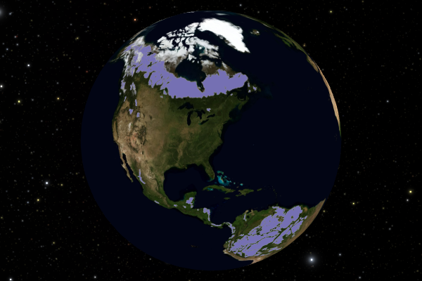
A biome is sort of a climactically and geographically similar area where communities of plants are found. You can have the same biome on different continents. We are looking at several forest visualizations. We will fly over the North Pole to see the boreal forest, a great coniferous forest adapted to the very short summers and long, cold winters. And it’s like a dark green wreath around the northern latitudes of the planet.

Just below the boreal biome are the forests that we are more familiar with. You can see temperate forests all the way across Eurasia and here, moving closer to home. Temperate forests, on the very broad basis, climactically and geographically speaking, are similar to one another, compared to tropical forests. Tropical forests are adapted to much more regular day-length, much more stable temperatures. And here, just for the sake of brevity, we have merged a whole bunch of different tropical forests together— sub-tropical and tropical, and wet and dry—just to give you an idea of these broad classifications of different types of forests on the planet. Each is adapted to its settings on the dials of temperature, precipitation, and fire.

Uniview cues
Browser Control: (2.Fires + Forests tab)
Load Layerset #2 button
Biomes:
Boreal Toggle button
Biomes OFF button
Tropical Toggle button
Biomes OFF button
Temperate Toggle button
Biomes OFF button
Biome Legend:
Legend Toggle button
Optional Borders:
US States Toggle button
Geoscope Layerset:
Load wvn11_dmns_2_FINAL.layerset
Sources

Biomes from the World Wildlife Fund (WWF; http://worldwildlife.org/biomes), with layers processed by Cynthia Powell.

wvn11_boreal_taiga.kmz

wvn11_all_tropical_subtropical.kmz

wvn11_all_temperate.kmz

wvn11.cc_biomes_legend.jpg

http://worldwildlife.org/biomes

Scene 3.70, frame 1
Scene 3.70

8000 Years Ago

Global Forests

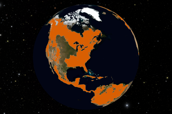
Collectively, all forests were distributed across vast regions of the planet until very recently in evolutionary time. We want to understand what forest cover looked like before the hand of man, before human activity modified the landscape. The World Resources Institute (WRI) has reconstructed the extent of forests on Earth from 8000 years ago. Compared to what we just saw, there are much greater expanses of forests that covered the planet. Huge parts of the planet that we no longer associate with forest are shown as forested.

Uniview cues
Browser Control: (2.Fires + Forests tab)
Original/Frontier/Working Forests:
Original Toggle button
Forests OFF button
Optional Borders:
US States Toggle button
Sources

World Resources Institute (WRI; http://www.wri.org/map/state-worlds-forests) layers processed by Cynthia Powell.

original_lost2.kmz

http://www.wri.org/map/state-worlds-forests

Scene 3.72, frame 1
Scene 3.72

Frontier Forests of Today

And so we ask today, what of these forests, the sort of intact forests that existed in prehistoric times, are left? The World Resources Institute has created a classification of what they call frontier forests. These are ecologically intact forests that have their full complement of top predators. These are truly intact forests without human intervention, where you can go see what the forest was like thousands of years ago.

What’s left in North America of the frontier forests? The boreal forest in the remote northern region is still our largest intact forest. But there are four little places in the U.S., four ancient forest heartbeats that remain.

Two of these represent some of our most celebrated national parks. This is Yellowstone National Park and this is Glacier National Park. What this tells us is the value of the investment we have made in protecting Yellowstone and Glacier. These are part of the remnants of truly intact parts of the forest that have ecological integrity reflecting ancient forests.

Uniview cues
Browser Control: (2.Fires + Forests tab)
Original/Frontier/Working Forests:
Frontier Toggle button
Forests OFF button
Optional Borders:
US States Toggle button
Uniview Controls:
Fly up to Yellowstone NP and Glacier NP in North America.
Sources

World Resources Institute (WRI; http://www.wri.org/map/state-worlds-forests)

layers processed by Cynthia Powell.

frontier.kmz

http://www.wri.org/map/state-worlds-forests

Scene 3.74, frame 1
Scene 3.74

Working Forests of Today

Of course we know that there are a lot more forests in this landscape and World Resources Institute has put together a working forests layer. We can argue about the definitions, but these are essentially forests where the hand of man is visible. We manage them. We have eliminated some of the top members of the food chain. These are forests that work and serve us.

Uniview cues
Browser Control: (2.Fires + Forests tab)
Original/Frontier/Working Forests:
Working Toggle button
Forests OFF button
Optional Borders:
US States Toggle button
Sources

World Resources Institute (WRI http://www.wri.org/map/state-worlds-forests)

layers processed by Cynthia Powell.

current_working.kmz

http://www.wri.org/map/state-worlds-forests

Scene 3.76, frame 1
Scene 3.76

Lost Forests of Today

And so if we put the commercial forest layer back up, then what’s left is the layer of forests that’s lost. These are landscapes that used to be forested, but where forests no longer exist. But it’s fascinating to think about this, because if forests existed here, if the conditions of temperature and precipitation and fire existed in the recent past for forests to be there, maybe our understanding of lost forests in existence can help inform our forest frustration practices.

Uniview cues
Browser Control: (2.Fires + Forests tab)
Original/Frontier/Working Forests:
Lost Toggle button
Forests OFF button
Optional Borders:
US States Toggle button
Sources

World Resources Institute (WRI; http://www.wri.org/map/state-worlds-forests)

layers processed by Cynthia Powell.

lost_minus_working.kmz

http://www.wri.org/map/state-worlds-forests

04

Continental: North American Forests

4 scenes
Scene 4.10, frame 1
Scene 4.10

Temperate North American Forests

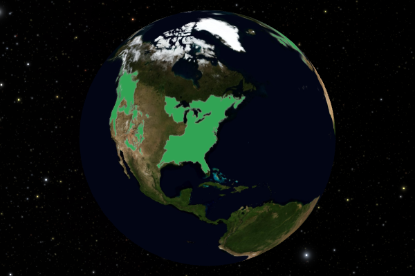
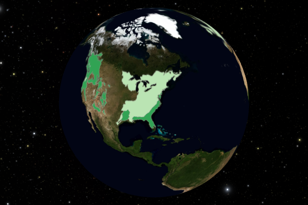
Let us look at the temperate forests that exist just across the U.S. We will break them down into another couple categories. There are the temperate coniferous forests, mostly evergreen forests of the west that we are used to in Colorado. And then there are the broadleaf forests, the deciduous forests of the east (that is, the forests that lose their leaves).

Uniview cues
Browser Control: (2.Fires + Forests tab)
Biomes:
Temp Broad/Conif Toggle button
Biomes OFF
Optional Borders:
US States Toggle button
Sources

Temperate Broadleaf and Temperate Coniferous from World Wildlife Fund (WWF; http://worldwildlife.org/biomes), with layers processed by Cynthia Powell.

wvn11_temperate_broadleaf.kmz

wvn11_temperate_conifer.kmz

50m-admin_UnitedStates_no_labels_white.kmz

CO_Counties.kmz

http://worldwildlife.org/biomes

Scene 4.20, frame 1
Scene 4.20

Longleaf Pine (Past and Present)

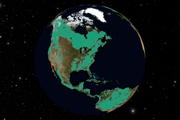
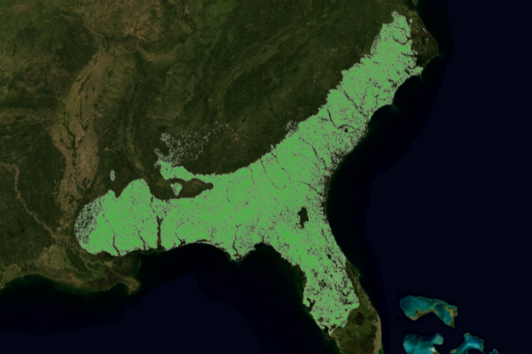
There is a unique isolated southeastern coniferous forest ecosystem. The organization NatureServe has painstakingly reconstructed the original extent of the longleaf pine ecosystem of the U.S. When the first explorers saw the longleaf pine, they called it “a vast forest of the most stately pine trees that can be imagined planted by nature at a moderate distance”. This was an intensely fire driven landscape and it covered 90 million acres of the southeastern U.S.

NatureServe has also given us an understanding of what the current extent of longleaf pine forest is. It is the most disappeared ecosystem in North America. There’s only 3% of the native longleaf pine left. But it is important to understand exactly where that is. What are the patches? How are they distributed? This kind of data is essential to understanding how to manage and conserve the remaining forest.

What has replaced the longleaf pine ecosystem? We can turn the working forest layer back on and recognize that the southeastern forests are working for us. This is where we get construction materials and paper products. We have working forests all across the southeast. The original ecosystem has been transformed into a forested ecosystem for human needs.

Uniview cues
Browser Control: (2.Fires + Forests tab)
Longleaf:
Historic Toggle button
Current Toggle button
Optional Borders:
US States Toggle button
Sources

NatureServe Landscope (http://www.natureserve.org/projects/landscope.jsp) data contributed by Regan Lyons Smith, Lori Scott, and Rickie White, and compiled by Cynthia Powell.

wvn11_longleaf_pine_current.kmz

wvn11_longleaf_pine_historic.kmz

landscope.jsp

Scene 4.30, frame 1
Scene 4.30

Ponderosa Pine (Past and Present)

Here we see ponderosa pine again historically reconstructed by NatureServe. The data show us a scattered distribution across a huge range of the western landscape. Mid-elevation pine is often found as the forest in wildland-urban interfaces (WUI).

While ponderosa pine has been reduced, that is nothing when compared to the longleaf pine. Ponderosa pine still covers much of western North America, and is an integral part of forests managed on public and private lands.

Uniview cues
Browser Control: (2.Fires + Forests tab)
Ponderosa:
Historic Toggle button
Current Toggle button
Optional Borders:
US States Toggle button
Sources

NatureServe Landscope (http://www.natureserve.org/projects/landscope.jsp) data contributed by Regan Lyons Smith Lori Scott, and Rickie White, and compiled by Cynthia Powell.

wvn11_ponderosa_pine_current.kmz

wvn11_ponderosa_pine_historic.kmz

landscope.jsp

Scene 4.40, frame 1
Scene 4.40

Land Cover

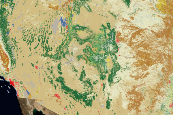
Of course we are just showing you the very most coarse classifications of different forests. But we all know that our natural heritage is much more diverse than this. So we want to show you what we think is almost more art than data. It’s the National Land-Cover Database and it uses reflectance of the ground as measured by satellites to classify 20 different types of vegetation and landscape that can be seen from space.

You will recognize much of the coniferous forests, and the little bit of mixed forests. This is a more refined division of what our landscape looks like, and a reflection of the diversity of our natural heritage.

Uniview cues
Browser Control: (2.Fires + Forests tab)
Earth:
NLDC 2006 Toggle button
Sources

National Land-Cover Dataset identifies 20 different land cover classes in the U.S. The data are derived from 30-meter Landsat Thematic Mapper data

(http://www.mrlc.gov/nlcd2006.php). A legend for the colors can be found here, and a full description of the metadata can be seen here.

ornldaac_ds10009.kmz

nlcd2006.php

here

here

05

Regional: North American Climate

3 scenes
Scene 5.10, frame 1
Scene 5.10

Forests of Western North America

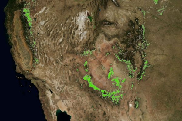
Now we travel to the forests of the western U.S., to look at the forested landscape and understand more about how it has changed recently. These are the forests that are the most familiar to us: the lodgepole pines, spruces, or firs. This will again be a dataset that we can see from space measuring the amount of forest cover. These are essentially the forests that we recognize today in our backyards.

This is the forest that we’ve been managing intensely for about 150 years. We’ve been harvesting it, clearing it, and suppressing fires within it. Where fires once naturally ignited and kept these forests pretty open, we practice forest fire suppression which has created dense stands of trees. We know that management has changed these forests quite dramatically.

But we know also that other things are changing about these forests. The climate is changing, for example. All of you in the room probably recognize that winters have been getting much milder in North America. We want to look a little bit how climate has been changing across this landscape as well.

Uniview cues
Browser Control: (2.Fires + Forests tab)
NA Western Forests Toggle button
Optional Borders:
US States Toggle button
Sources

NASA MODIS Vegetation Continuous Fields (VCF). Data contributed by John Townshend and http://modis-land.gsfc.nasa.gov/vcc.html and compiled by Cynthia Powell.

wvn11_forest_cover_westernNA.kmz

vcc.html

Scene 5.20

Changing Climate of Western North America

Is there a signal of climate change in our landscapes that our forests are experiencing? If so can we identify the nature of these changes, so we can better understand how to cope with them?

Uniview cues
Browser Control: (3a.Drought, Beetles tab)
Load Layerset #3 button
Geoscope Layerset:
Load wvn11_dmns_3_FINAL.layerset
Scene 5.25, frame 1Scene 5.25, frame 2
Scene 5.25

January Minimum Temperatures

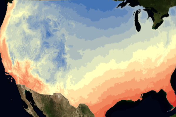
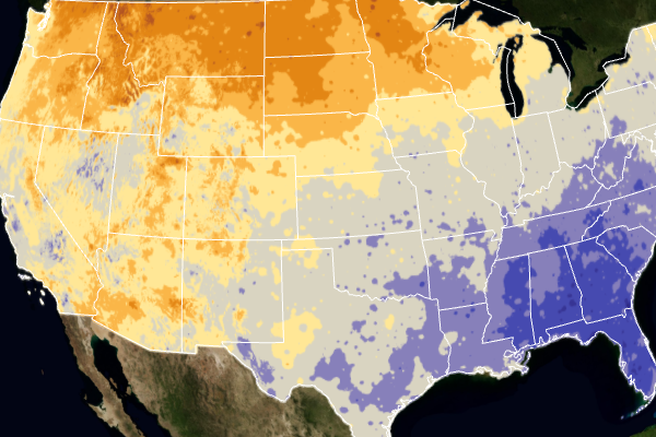
This is a dataset that tells us that winters are getting milder. This shows January minimum temperature differences between the last decade and the 20th century. So if you had a thermometer in your backyard and you were measuring January minimum temperature, and you looked at the difference in the last decade as compared to the 20th century average, you would see almost five degrees of January minimum temperature increase in the northern latitudes.

We see that it’s actually getting a little bit cooler in January minimum temperatures in the southeast. We see the west is getting hotter than the east. The north is getting hotter than the south. And the mountains are getting disproportionately warm relative to the lowlands.

This is a map of actual changes in January minimum temperatures. Not climate models, but analysis you could have done if you started measuring January minimum temperature with your backyard thermometer in 1900.

Uniview cues
Browser Control: (3a.Drought, Beetles tab)
Load Layerset #3 button
PRISM Data
Delta Temp Toggle button
1901-1980 Baseline Toggle button
2001-2010 Warming Toggle button
1 Std Dev Toggle button
Sources

Oregon State University PRISM 800m analyzed by Healy Hamilton’s Lab.

CP checking delta temps, the 1901-1990 baseline, and the

2001-2010 temperatures.

2001-2010 minus 1901-1980 (delta) Jan delta min temp high 5.6 C low -3.4 C

1901 to 1980 Jan tmin high 18.6 C low -24.5 C

2001 to 2010 Jan tmin high 17.4 C low -21.8 C

d_tmin_1.kmz

s1_tmin_1.kmz

tmin_1_10yr.kmz

tmin_1_baseline.kmz

06

Regional: Drought

1 scene
Scene 6.10, frame 1
Scene 6.10

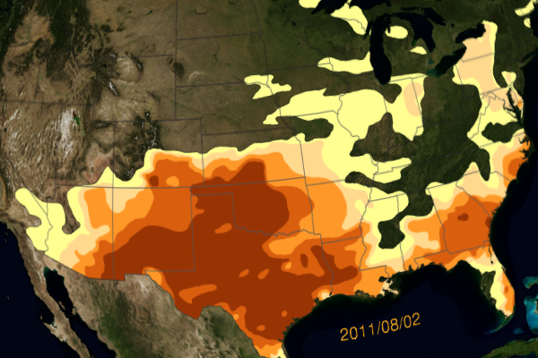
And it’s not only minimum temperatures that are changing. We also know that at the same time warming is occurring, that western forests are experiencing cycles of drought. We have data from the National Drought Monitor Index that shows one week in summer for the last ten years. The more intense drought is the darker brown and the less intense drought a lighter brown. But what we can see as we cycle through the years, is that every single year somewhere in western forests, a drought is occurring. We see cycles of drought as they occur across the western forest landscape.

So the combination of warming winters, drought stress, and fire suppression have pushed western forests outside the range of their natural cycles. And we’ve been witness to these changes. We hear about it in the news all the time. One way that these changes are expressed is an imbalance in the relationship between western forests, and one type of their natural inhabitants: the bark beetles.

Uniview cues
Browser Control: (3a.Drought, Beetles tab)
Load Layerset #3 button
Drought Monitor
Reset Cycling button
Continuous Cycling button
2000, 2001, 2002, 2003, 2004, 2005, 2006, 2007, 2008, 2009, 2010, 2011, 2012, Recent, buttons
Legend Toggle button
ALL OFF button
Optional Borders:
US States Toggle button
Geoscope Layerset:
Load wvn11_dmns_3_FINAL.layerset
Sources

Further resources on drought can be found at the U.S. Drought Portal (www.drought.gov/drought/) and the U.S. Drought Monitor (droughtmonitor.unl.edu). Weekly drought maps are archived at droughtmonitor.unl.edu/DataArchive/GISData.aspx

usdm000801.kmz

usdm010807.kmz

usdm020806.kmz

usdm030805.kmz

usdm040803.kmz

usdm050802.kmz

usdm060801.kmz

usdm070807.kmz

usdm080805.kmz

usdm090804.kmz

usdm100803.kmz

usdm110802.kmz

usdm120807.kmz

usdm130528.kmz

wvn11.cd_drought_legend.jpg

www.drought.gov/drought/

droughtmonitor.unl.edu

droughtmonitor.unl.edu/DataArchive/GISData.aspx

07

Regional: Bark Beetles

1 scene
Scene 7.10, frame 1
Scene 7.10

Bark beetles have evolved as a native component of our forests. But the environmental changes that we have just discussed have been favoring the life cycle of the beetle. Over the last 15 years, the U.S. Forest Service has been carefully observing the distribution of beetle-damaged forests.

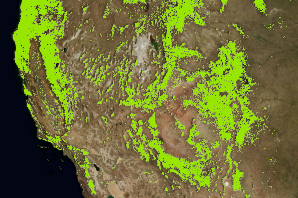
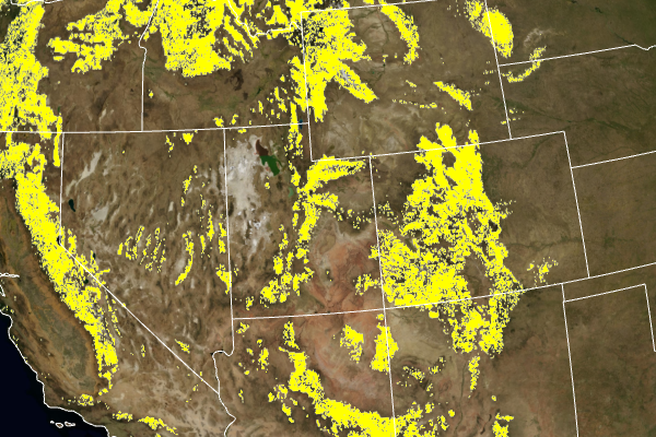
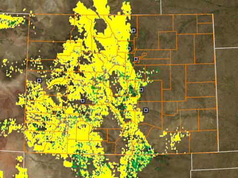
We are watching year by year, beginning in the mid-1990’s the results of aerial over-flights, where trained observers have recorded damaged forests. Year after year they are mapping where the damaged forests can be seen from the air at the highest spatial resolution that they can. These are forests that are discolored, and are sick in some way. They’re not all uniformly dead. The forests pushed into a state of stress are being influenced by the cycles of bark beetles who are favored by current conditions. This is the cumulative map, not including British Columbia, of beetle infested forests. Essentially this map mirrors the maps we’ve seen of the distribution of the western coniferous forests. Almost everywhere across the west, there have been cycles of beetle damage.

We’re going to spend some time now in Colorado, and take a closer look at how the cycles of forests and beetles and change have been affecting local parts of Colorado. We will explore the local version of the phenomenon that we now understand is occurring at the scale of the continent.

Uniview cues
Browser Control: (3a.Drought, Beetles tab)
Load Layerset #3 button
Lodgepole Beetle Impact
1997, 1998, 1999, 2000, 2001, 2002, 2003, 2004, 2005, 2006, 2007, 2008, 2009, 2010, 2011, 2012, Cumulative US, Cumulative US+BC, buttons
ALL OFF button
Optional Borders:
US States Toggle button
Geoscope Layerset:
Load wvn11_dmns_3_FINAL.layerset
Sources

USFS Aerial Detection: Annual pine beetles area affected in the continental US (CONUS) during the years 1997-2012 (individual KMZ time series), along with cumulative pine beetles in CONUS 1997-2012.

1997.kmz

1998.kmz

1999.kmz

2000.kmz

2001.kmz

2002.kmz

2003.kmz

2004.kmz

2005.kmz

2006.kmz

2007.kmz

2008.kmz

2009.kmz

2010.kmz

2011.kmz

2012.kmz

cumulative.kmz

wvn11_forest_cover_westernNA.kmz

08

Local: Impacts from Drought and Beetles

11 scenes
Scene 8.05, frame 1Scene 8.05, frame 2Scene 8.05, frame 3
Scene 8.05

Regional Distribution of Trees

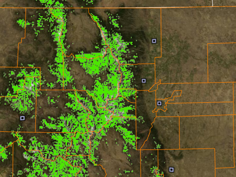
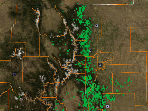
We start with a topographical map illustrated using LANDSAT data, and overlay it with different kinds of tree species in our forest. We can turn on pixels indicating the distribution of lodgepole pines, which are concentrated in the northern part of Colorado, and are a sort of turquoise color. A similar dataset of the distribution of spruce trees will show up in a different shade of green. The ponderosa pines extend out into the Black Forest area, just illustrating one more species of tree. You can see them extending out into the areas we live on the eastern plains.

Thus in the forests of Colorado and Wyoming, there is a blend of different kinds of trees. Of course there are fir trees, Pacific cone pine trees, and a variety of other trees. The forest is not homogeneous, but is comprised of different species, and where they live is a function of latitude, altitude, slope orientation, soil characteristics, etc.

And in this mosaic of different kinds of trees, the trees have been subjected to attacks by a variety of species of beetles. Beetles are of different species attacking different trees in different ways.

Mountain pine bark beetle prefers the lodgepole pines, focusing in the northern part of the state of Colorado, and extending on up to the north. The epidemic of mountain pine bark beetles actually peaked about 2008 in the Grand County, North Park, and Middle Park areas. They are extending across the Front Range coming into Larimer and Boulder Counties. The mountain pine bark beetle also can eat the ponderosa pines, which are being attacked in Larimer County in particular.

Uniview cues
Browser Control: (3a.Drought, Beetles tab)
Load Layerset #3 button
Lodgepole Toggle button
Spruce Toggle button
Ponderosa Toggle button
Optional Borders:
US States Toggle button
CO Counties Toggle button
Geoscope Layerset:
Load wvn11_dmns_3_FINAL.layerset
Sources

Data from Landfire for all western US (http://landfire.cr.usgs.gov/viewer/viewer.html?bbox=-108.882653409426,35.4328843893838,-104.177922635156,41.7017142886605); extracted and compiled by Cynthia Powell.

lodgepole2_v3.kmz

spruce.kmz

wvn11_ponderosa_pine_current.kmz

wvn11_ponderosa_pine_current_v3.kmz

viewer.html

Scene 8.06, frame 1
Scene 8.06

Distribution of Beetles and Trees

If we turn back on the spruce trees and the lodgepole pines, and then overlay the cumulative beetles. We see that the overlay maps the distribution of the trees extremely well. Remember that the yellow in the cumulative overlay does not indicate the entire death of the forest, but it does indicate impact, and that impact is regional in scale.

As we look at these assembled datasets of varying scales, we can appreciate that the hand of man has been etched on many of the working forests in the western part of the U.S., but also probably less so as we move up north into Canada and into parts of Alaska.

Nonetheless, between cutting down the timber about a 120 years ago for use for fuel, for mine timbers, and railroad ties, we have substantially modified many of these forests. They have since re-grown to be relatively uniformly after that cutting episode.

There has been fire suppression here since the National Forest Service was established, the so-called 10 a.m. fire limit. Forest fires were all supposed to be put out by 10 a.m. It was a vigorous effort to suppress fires. Again this was the case mostly in the National Forests of the western part of the United States, but less so going up into Canada.

And from the drought series shown earlier, this area has had droughts sporadically over the last twenty years. Those droughts have encompassed sub-regional areas, with areas that have experienced some relief from drought over time. The drought, the history of fire, and forest management are overlaid by the regional pattern of warming, which transcends everything, and extends well up into the Arctic.

Uniview cues
Browser Control: (3a.Drought, Beetles tab)
Load Layerset #3 button
Lodgepole Beetle Impact Cumulative US+BC button
Optional Borders:
US States Toggle button
CO Counties Toggle button
Geoscope Layerset:
Load wvn11_dmns_3_FINAL.layerset
Sources

Beetle impact data from USFS Aerial Detection.

Time series created by Arjan Meddens (University of Idaho, Moscow, ID), and

compiled by Cynthia Powell.

Meddens, A, et al. 2012, “Spatiotemporal patterns of observed bark beetle-caused tree

mortality in British Columbia and the western United States,” Ecological Applications, 22(7), 2012, pp. 1876–1891.

cumulative.kmz

Scene 8.10, frame 1Scene 8.10, frame 2
Scene 8.10

Wildfires

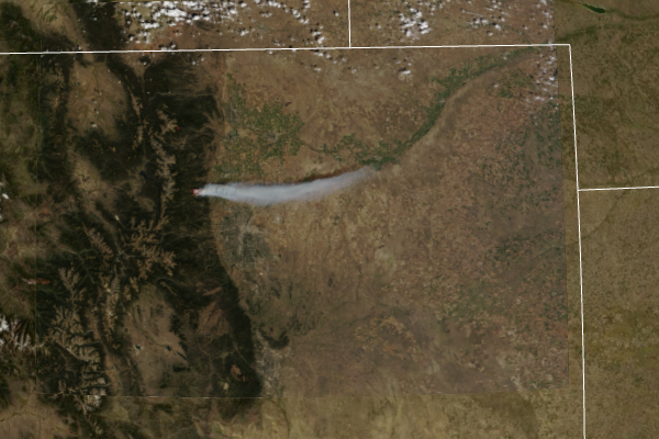
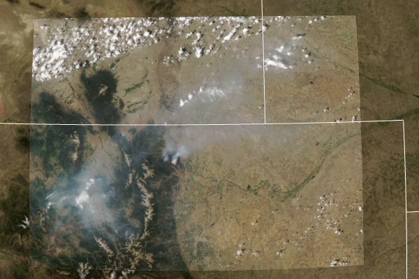
The natural cycle of fire includes recent fires with smoke plumes stretching across the state that can be seen via satellite imagery from space.

The first image is from the Fourmile Canyon fire outside of Boulder, in September 2010. The second is from the High Park fire outside of Ft. Collins in June 2012.

Uniview cues
Browser Control: (3b.Panos & Slides tab)
MODIS
Toggle buttons
Optional Borders:
US States Toggle button
CO Counties Toggle button
Sources

Fourmile Canyon fire image is from MODIS instrument on the Terra satellite, captured at 12:15pm local time, 6 September 2010. The red outline represents the area with high surface temperatures associated with the fire. (http://earthobservatory.nasa.gov/NaturalHazards/view.php?id=45675)

The High Park fire image was captured by the MODIS instrument on the Aqua satellite, captured at 1:40pm local time, 18 June 2012. (http://earthobservatory.nasa.gov/NaturalHazards/view.php?id=78312)

FourmileCanyonFire.kmz

HighParkFire.kmz

view.php

view.php

Scene 8.25, frame 1
Scene 8.25

Mountain Pine Beetle

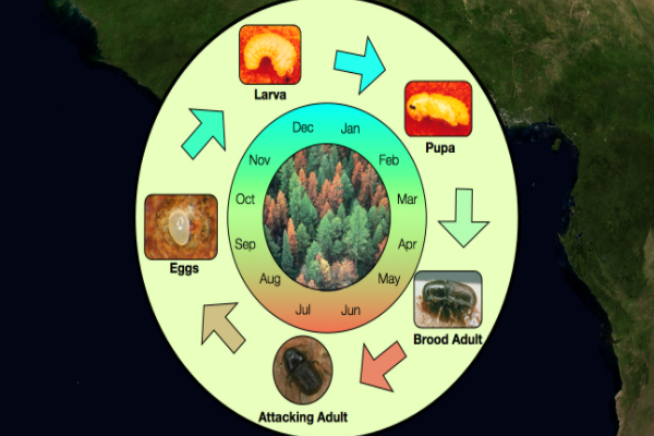
The mountain pine attacks trees by burrowing into them as adults. Once inside a pine tree, adult beetles lay eggs in the fall. These hatch into larva and turn into pupae through the winter, before finally growing into the next generation of adults. Only for a short period of time during the summer do the adults emerge from the tree it grew from and fly to spread to new trees.

What kills the trees is the blue stain fungus introduced by the beetle. The fungus prevents the tree from introducing sap which can repel beetles, and will also block water and nutrient transport inside the tree. As the tree dies, its pine needles will turn red, and then eventually turn gray as the needles fall off.

The pictures show stands of red trees, slowly dying because of the beetles. In the winter snow, gray trees are easy to spot. Note the few living green trees interspersed among the gray stands of pines. Some of the trees attacked by beetles can be seen generating sap to push out the burrowing beetles. Peeling the bark away from a dead or dying tree can also reveal the burrows made by the beetles.

In Colorado, there have been attempts to clear the felled trees from the landscape. Dying and dead trees are removed when they are near roads or highways, and thus could be dangerous to travelers. Downed trees are piled up to be burned in the winter.

Uniview cues
Browser Control: (3b.Panos & Slides tab)
forest:
Road 1, Road 2, Side View buttons
Pine Beetle:
Close-Up, Life Cycle buttons
Beetle Effects:
Sap on Bark, Tracks in Wood, View 1, View 2, View 3, Wood Pile, Logging Truck, Ground 1, Ground 2, Holes, Sap, Wood Pile 1, Wood Pile 2 buttons
Winter:
Side View 2, Side View 3, Vista buttons
ALL SLIDES OFF button
Scene 8.30, frame 1
Scene 8.30

Beetle-kill Impacted Forests

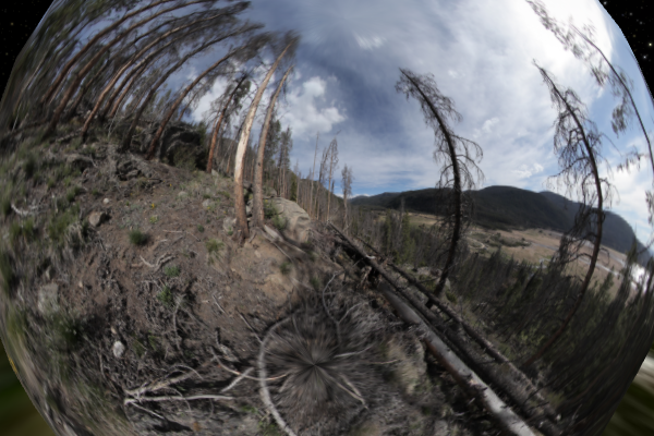
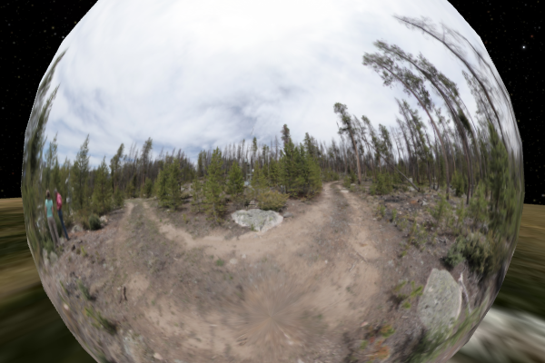
Bob Raynolds and Ka Chun Yu went up to Lake Granby at the edge of Rocky Mountain National Park to see what a dead or dying forest looks like. The forests in Grand County have been very severely hit by the mountain pine bark beetle.

In the distance is a view of the relatively dry reservoir Lake Granby, which is part of the system that drains water from the upper reaches of the Colorado River system, pumps it across the Continental Divide (underneath Estes Park and Rocky Mountain National Park) to the Front Range as part of the Colorado Big Thompson Project.

In the forest were indeed many dead trees. As the needles fall from the trees, they go from the red to the gray stage.

The challenging mountainous landscape in the panorama is a wilderness area, where chain saws are not allowed. And trees are starting to fall down—in fact, the number often cited for Colorado is that 100,000 trees per day fall down in Colorado. The lodgepole pine tree has substantial root systems, and so once the tree dies, the roots are cut off and unable to hold the tree up. Then the trees topple.

The mature tall trees can suffer from wind damage once other trees fall over, and the standing isolated trees are exposed to the wind. And so, as you move into the wilderness areas, the toppled trees become obstacles to navigation. And it’s one thing for people to move over the fallen logs; it would be even more challenging for a horse or llama. And because chain saws are not allowed, you would need to hand-cut all of these lodgepole pick-up-sticks.

The forest has lots of dead trees. Many fallen trees are visible in the foreground. With fewer needles in the trees, the forest can be seen more clearly. However you notice that once in the forest, not all the trees are dead. In the middle of this dying forest that is mostly impacted by the beetles, somewhere between 20-30% of the trees are still alive.

But as we look over towards the right, I’ll just draw your attention, we can see through the dead trees the living trees are showing up. From a distance, the forest appears awfully grim, but once you get into the forest you can see that there are trees that have survived, whether they are resistant to the beetles, or the beetles were distracted by some other tree. We are not sure why, but some trees did survive.

Uniview cues
Browser Control: (3b.Panos & Slides tab)
Panos
Roaring Fork Trail 4 Fly To/Jump To buttons
Object Tree:
Earth→DMNS-Ka Chun Yu→Roaring Fork Trail 4
Sources
Scene 8.35, frame 1
Scene 8.35

At the Visitors Center at the gateway to the west side of Rocky Mountain National Park, is one of the thermometers mentioned earlier. This panorama shows the weather station, which has been recording data since the tail end of the 1940s. It’s one of the most long-lived weather stations without any urbanization whatsoever anywhere near it.

The weather station used to be in a mature lodgepole pine forest. It’s now in a clearing, because the Park Service had to chop down the dead and dying trees because they were afraid they were going to fall over and crush the weather instruments.

But again, with the dead trees removed, you can see the living forest. There are many small lodgepole pines, maybe 10-15 years old. They are the forest of the future.

As the trees fall, the forests will change dramatically. The trees are regenerating. The future forest will come. This is not just a story about extinction.

Uniview cues
Browser Control: (3b.Panos & Slides tab)
Panos
Weather Station Fly To/Jump To buttons
Object Tree:
Earth→DMNS-Ka Chun Yu→Weather Station, Kawuneeche Visitors Center, RMNP
Sources
Scene 8.40, frame 1
Scene 8.40

Temperatures

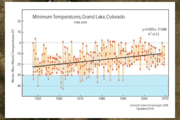
Here is a plot of temperature from this thermometers, from Colorado State University’s Colorado Climate Center. The red dots represent the coldest temperature recorded during the winter months (or November, December, January, February and March). There is a cluster of five data points for each year, or each winter. And as you move from 1948 up to almost the present, you will see a gradual increase in minimum winter temperatures described on the earlier large-scale map. Here you are seeing one data point of that bigger map.

The mountain pine beetles can be killed in the early winter by slightly warmer temperatures. But in the depth of winter, they develop antifreeze in their larva, and temperatures have to drop to -30 degrees Fahrenheit to do them in. From this plot, between 1990-2010, there were no occurrences of -30 degrees Fahrenheit temperatures. So the beetles took the opportunity to spread across our landscape in central Colorado. We can see the data recorded at this site has led to the results visible in the forest.

Uniview cues
Browser Control: (3b.Panos & Slides tab)
Panos
Weather Station Fly To/Jump To buttons
Grand Lake Temp: 1948-2009 button
ALL SLIDES OFF button to turn off
Sources

Data from Colorado State University’s Colorado Climate Center. Graph prepared by Bob Raynolds.

wvn11.bc_GrandLake_Temp_updated.jpg

Colorado Climate Center

Scene 8.45, frame 1
Scene 8.45

Effects of Drought at the Local Level

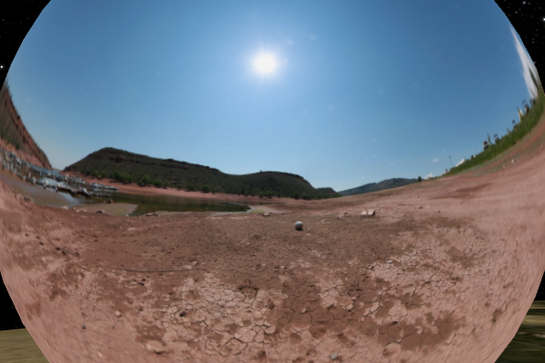
We can emphasize that the conditions of drought severely impacted people in Colorado. This panorama of Horsetooth Reservoir, which holds water for the Fort Collins area, was taken last year. Ka Chun Yu and Bob Raynolds were in part of a marina that now has dried up. A boat float and a boat anchor are out on the muddy flats. Somewhere off in the distance is the water.

And what has occurred in Horsetooth Reservoir is mirrored in many other reservoirs today. Dillon Reservoir in the Frisco-Dillon area is like that, as are Lake Powell or Lake Mead. These systematic occurrences of conditions are a challenge to the western U.S. Although Colorado had a wet spring in 2013, much of the state is still short of snow. These kinds of conditions may be more and more common as we go into the future.

Uniview cues
Browser Control: (3b.Panos & Slides tab)
Panos
Horsetooth Reservoir Fly To/Jump To buttons
Object Tree:
Toggle on Earth→DMNS-Ka Chun Yu-Lucy Conklin→Horsetooth Reservoir→Marina 1
Sources
Scene 8.50, frame 1
Scene 8.50

Run-off in Aftermath of Forest Fires

We next look at the effects of flowing water in fire-burned areas. This panorama shows the north end of the High Park fire outside of Fort Collins. In this catchment is drainage that drains down into the Cache la Poudre River. The landscape had been scoured by rainfall, after it had been burned in the High Park fire.

The debris flow had come down and eventually crossed the road, before going into the Cache la Poudre River. Locals will know that Fort Collins last year had potable water problems, because of the fire debris that went down into the public drinking water supply.

You can see that it flowed down the stream in the picture, with debris flow removing the bark from the trees. It took all the soil, the dust, the organic material, including all of the soot and charcoal, and the flow dumped down the Cache la Poudre River, where it flowed into the potable drinking water supplies. The water authorities in Fort Collins had to reallocate water from Horsetooth Reservoir and Carter Lake to avoid sending this water into the municipal supplies.

Uniview cues
Browser Control: (3b.Panos & Slides tab)
Panos
High Park Mud Slide 1 Fly To/Jump To buttons
Object Tree:
Toggle on Earth→DMNS-Ka Chun Yu-Lucy Conklin→High Park Fire→Mud Slide 1
Sources
Scene 8.52, frame 1
Scene 8.52

Forest Fires

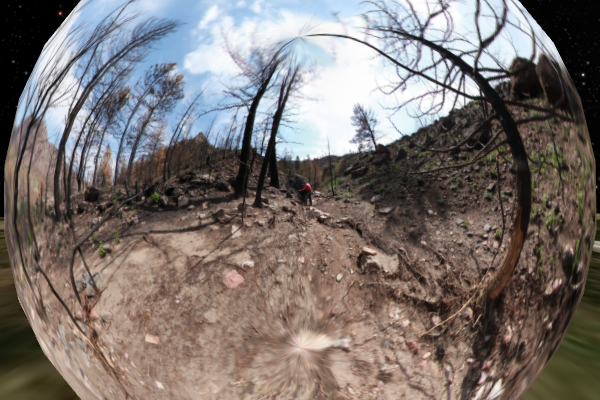
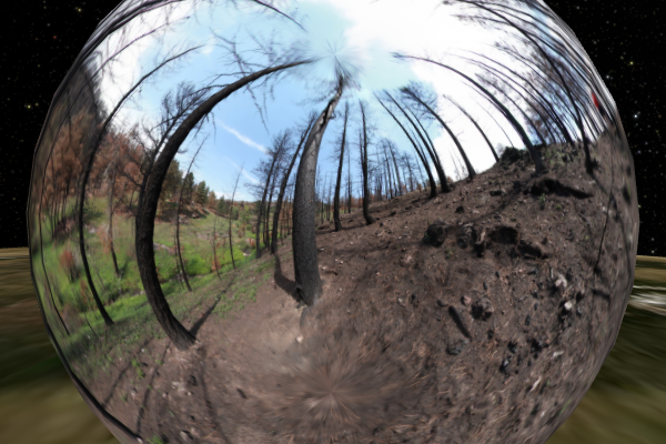
The next panorama shows the High Park fire again. We are in a severe burn scar area. The tongues of fire had licked the birds from the sky. It’s hard to believe but Bob Raynolds and Ka Chun Yu found bodies of birds here. The fire had been ferocious in this area. Life had been damaged and destroyed. But just across the way, we can see across a garden and a home. The trees are green. The grass is green. There are tomatoes on the plants.

So not only the beetles, but the fires have also created mosaic landscapes. These forests are in transition. We are seeing a new world, one that is a little unfamiliar on the one hand, but one that has wonderful opportunities for biodiversity to develop. There are lots of edge environments, with habitat areas that are between open areas and closed areas. These trees will fall over, and young trees will grow. And the landscapes of Colorado will change.

Uniview cues
Browser Control: (3b.Panos & Slides tab)
Panos
High Park on Slope 4 Fly To/Jump To buttons
Object Tree:
Toggle on Earth→DMNS-Ka Chun Yu-Lucy Conklin→High Park Fire→On Slope 4
Sources
Scene 8.54, frame 1
Scene 8.54

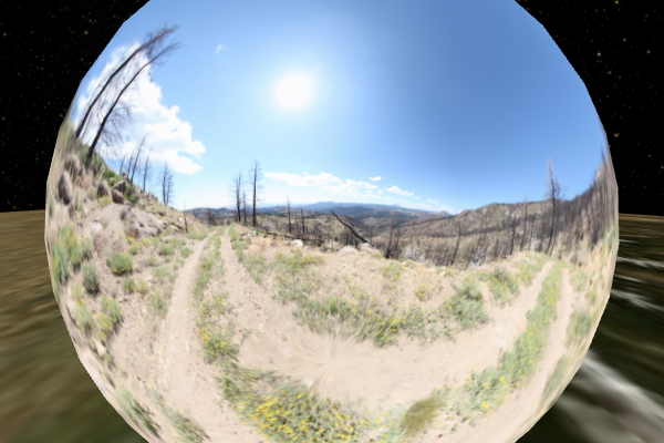
The last panorama shows an area from the Fourmile Canyon fire which burned in September 2010. The landscape again shows dead trees and a mosaic pattern in the distance, with a mix of burned and un-burnt areas.

Uniview cues
Browser Control: (3b.Panos & Slides tab)
Panos
Fourmile Canyon From Road 4 Fly To/Jump To buttons
Object Tree:
Toggle on Earth→DMNS-Ka Chun Yu→Fourmile Canyon Fire→From Road 4
09

Conclusions

4 scenes
Scene 9.10, frame 1
Scene 9.10

Peak Beetle

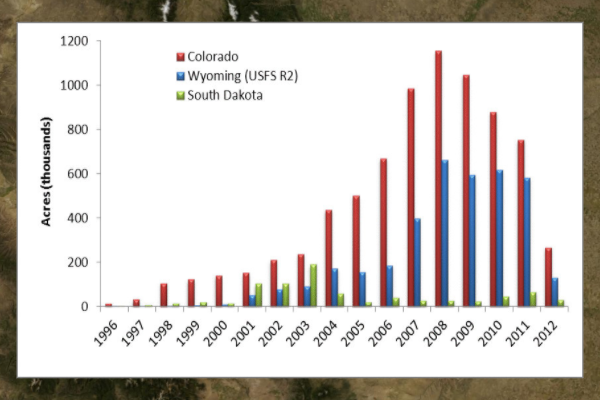
Colorado, Wyoming, and South Dakota has seen peak number of mountain pine beetles based on the number of acres of lodgepole forest impacted.

Uniview cues
Browser Control: (3b.Panos & Slides tab)
Peak Beetle: 1996-2012 button
ALL SLIDES OFF button to turn off
Sources

Data from the U.S. Forest Service. Graph prepared by Bob Raynolds.

wvn11.ae_peak_beetle_graph.jpg

Scene 9.20, frame 1
Scene 9.20

Bioregional Impacts in the Colorado Front Range

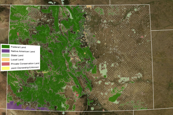
And as we look to the future, we have to look at what strategies we need to conserve and preserve lands. And this map illustrates the preserved lands of Colorado. It’s a wonderful opportunity to almost boast about what we’ve been able to do through the hard work of our predecessors in terms of conserving lands in Colorado.

North is to the top, and visible are the Elk Mountains in Wyoming, and the Front Range of Colorado. The greens are Federal lands: National Forests, and BLM land which characterize much of the Rocky Mountain side of the state. The pale blues are state lands (Section 16 lands, if you are familiar with the school sections out on the high plains). As we look more closely, the cities of Denver and Boulder are visible. There are additional conservative lands in the area of the foothills: park areas, city parks, public parks, and Open Space lands particularly concentrated in Boulder County. There is a tremendous amount of Open Space land preserved both in the foothills and on the plains.

A new movement that has taken place in the last couple of decades is developing conservation easements. Many of the yellow features on the eastern side of Boulder County are conservation easements where homeowners or landowners have designated that their land will not be subdivided, and will not be developed. The owners get certain tax benefits when the land is put into permanent conservation.

As you look at this kind of map we can take great pride in the fact that huge areas have been conserved. Many of them very long and contiguous which allows for corridors for the migration of species that may wish to migrate either north, or up, as conditions change.

These kinds of maps allow us to develop strategies for additional conservation efforts, and for additional land preservation initiatives. It allows us to sit back and strategize about how things have developed in the very pro-active County of Boulder. And maybe some of the patterns that are done in Boulder can be taken someday out to Weld County, Larimer County, and even Douglas County.

Rocky Flats and the Rocky Mountain Arsenal both show up as wildlife preserves. If you go to the Rocky Mountain Arsenal, you can see a bison herd and prairie dogs, and visit the beautiful visitors center. Visible are Lowry, Cherry Creek Reservoir, and Aurora Reservoir. We have a growing awareness of the preciousness of Open Space lands, and opportunities for species to regenerate and to develop. People are doing many of the right things and we can take solace from that.

Uniview cues
Browser Control: (3b.Panos & Slides tab)
CO Protected Areas Toggle button
Legend Toggle button
Sources

US Protected Areas Data (USPAD) downloaded from Databasin (http://databasin.org/) and compiled by Cynthia Powell.

wvn11_CO_protected_areas.kmz

wvn11.ce_CO_protected_areas_legend.jpg

http://databasin.org/

Scene 9.25

Strategies for Dead Trees

If we return to the dead tree story, you see that the wood biomass is being used as a resource. The blue stain wood has been used for decorative furniture. There are people going into the forest, salvaging the wood, and making wood pellets for wood stoves in Kremmling for instace, which has a big wood pellet facility. The wood pellets are being exported out of the United States.

Boulder County treats about 250 acres of their 30,000 acre Open Space lands and forest every year. By “treating,” we mean they are thinning trees out, to achieve what might be a more historic landscape scene with widely spaced trees. Less of the forest will be susceptible to fire and hopefully less of it to beetles. The woody material is salvaged and ground up, where it is then used to heat the Boulder County facilities. They are saving $20,000 a year in Boulder County using their wood biomass for heat in the winter.

There are strategies for using the wood. There are strategies for developing new industries associated with the wood. And of course, there are also strategies for recovery. The forest service and other agencies are involved in restoration and recovery efforts.

Sources

Steamboat Today article: “Kremmling wood pellet plant lands deal for dead timber on Routt National Forest.” and Longmont Times-Call article:

“Pine trees being chipped for Boulder County biomass boilers.”

“Kremmling wood pellet plant lands deal for dead timber on Routt National Forest.”

“Pine trees being chipped for Boulder County biomass boilers.”

Scene 9.27, frame 1
Scene 9.27

Tree Strategies for the Future

These are becoming movements worldwide. Wangari Maathai, the Nobel Prize winner from Kenya, has championed the planting of trees. Her tree plantations are visible in Kenya. In a forest north of Nairobi, the trees are only about three feet high, but there are 350,000 trees that had been planted on the African savannah. They say in ten years you will be able to have tea in the shade of the forest. Eucalyptus trees grow very quickly.

So we have the capacity to modify landscapes. We have the capacity to plant trees. Denver had the Million Tree Initiative that was set up by then Mayor Hickenlooper in 2006. The City of New York has a Million Tree Initiative as well. And we can plant trees and be involved in this too.

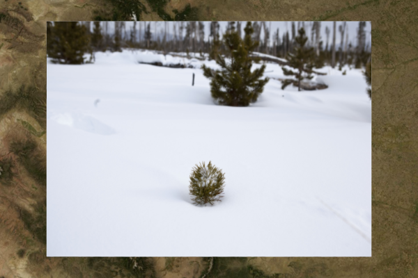
The final set of images are up by Gold Creek Pass taken in the winter of 2012-2013. Again the gray forest looks mostly dead. But if you look closely you will see the green trees. They are in there. The new forest is coming. The few isolated trees are full of pine cones, which are full of seeds. The young trees are growing. If you look closely, you will see an iconic little tree peeking out of the snow drifts here. This tree will one day also provide shade, and we will look forward to that.

Uniview cues
Browser Control: (3b.Panos & Slides tab)
Willow Creek:
Ranch Sign, Young Trees 1, Young Trees 2, Pine Cone 1, PIne Cone 2, Baby Pine buttons
ALL SLIDES OFF button to turn off
10

Credits

1 scene