Resilient Landscapes: The History and Future of Black Hills Floods

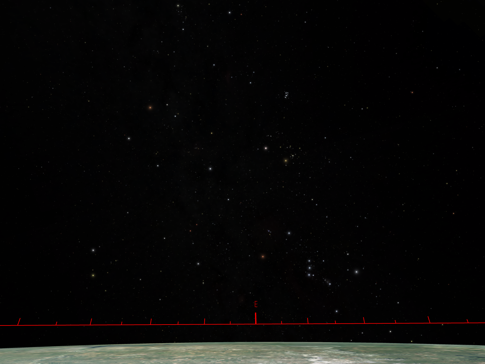
A view of the Night Sky: Where are we?

Studying sky across electromagnetic spectrum

In the modern era, not only have we continued to look at the sky, but we have used our latest tools to help us build a three-dimensional atlas of the Universe to allow us to understand it better.

Technological advances allow us to probe the electromagnetic spectrum beyond what is visible to our eyes. It is with these detectors that we find other connections with the cosmos.

In visible light, our Milky Way Galaxy, home to our Sun and hundreds of billions of other stars, appears as a bright band, broken up by dark dust clouds in the foreground that block star light in the background.

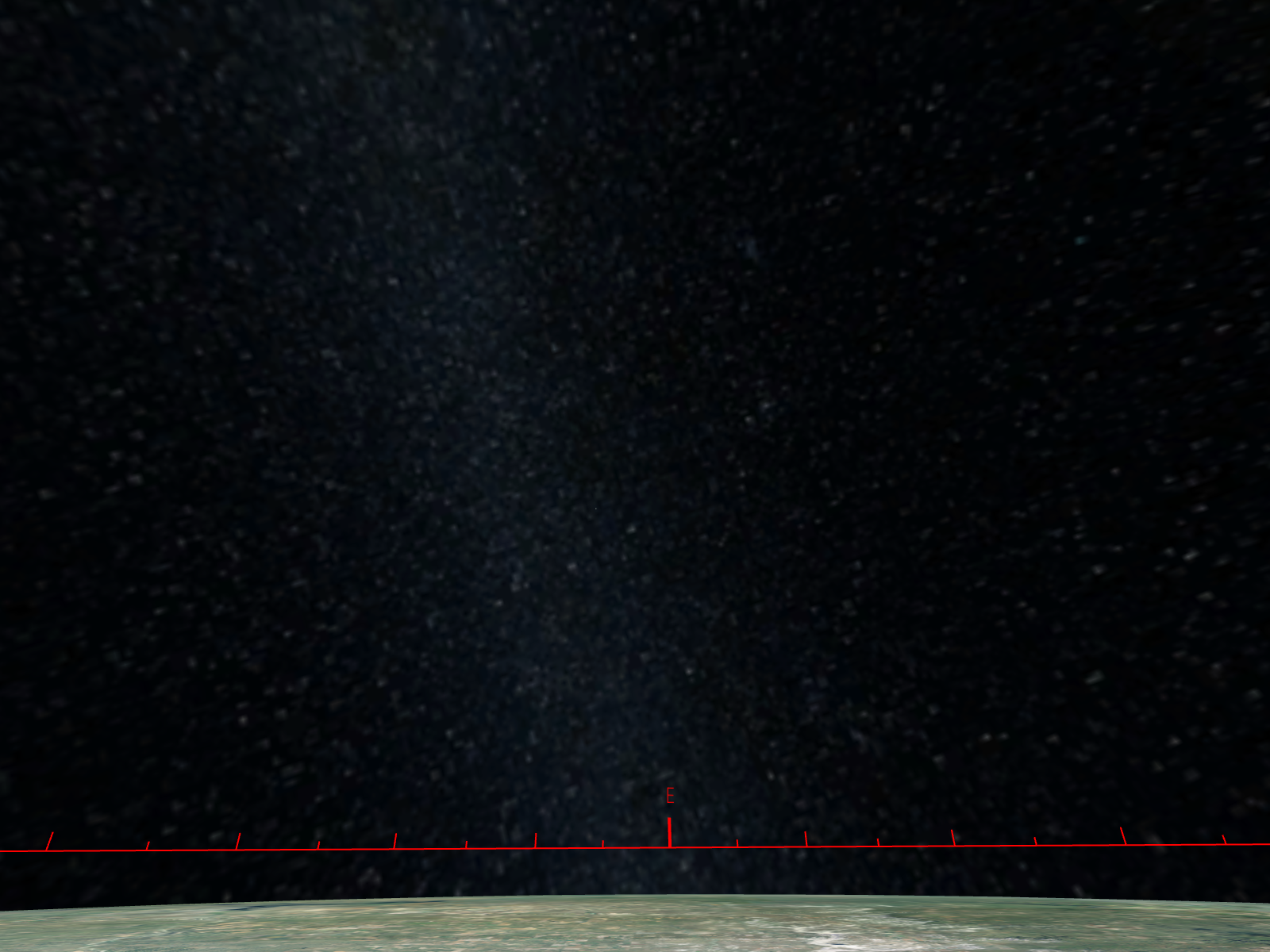
If we switch to viewing the sky in the near-infrared, the obscurations becomes transparent in many places. We can peer right through much of this gas and dust clouds, to see the band of cooler stars that lay beyond.

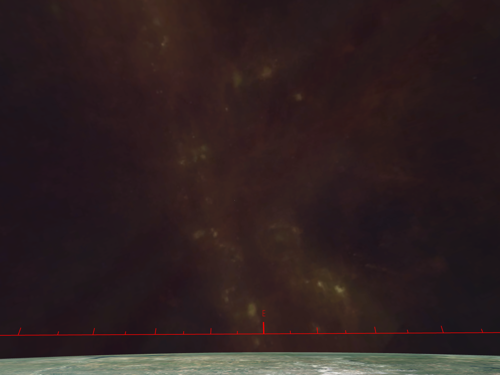
In the mid-infrared range we can see the wavelengths emitted by complex hydrocarbons which are commonly found in coal and interstellar gas clouds. We also see the red giant stars, planetary nebulae and massive stars so young that they remain deeply embedded in their parental molecular gas clouds.

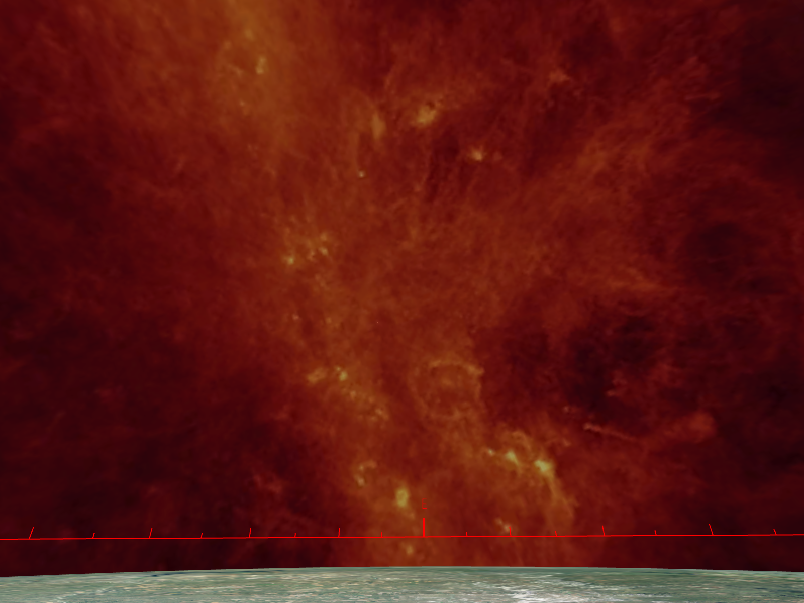
As we continue into the far infrared, the stars completely disappear since they emit little light at these wavelengths. Because they are relatively cold, the dust and gas clouds themselves start to glow in the far infrared. Most of what we see is emissions from the dust warmed by the absorbed starlight from stars embedded in the clouds.

We have learned that the cores of these clouds can collapse under their own gravity and form stars. It’s from something like these that our Sun and its family of planets was born 4.5 billion years ago.

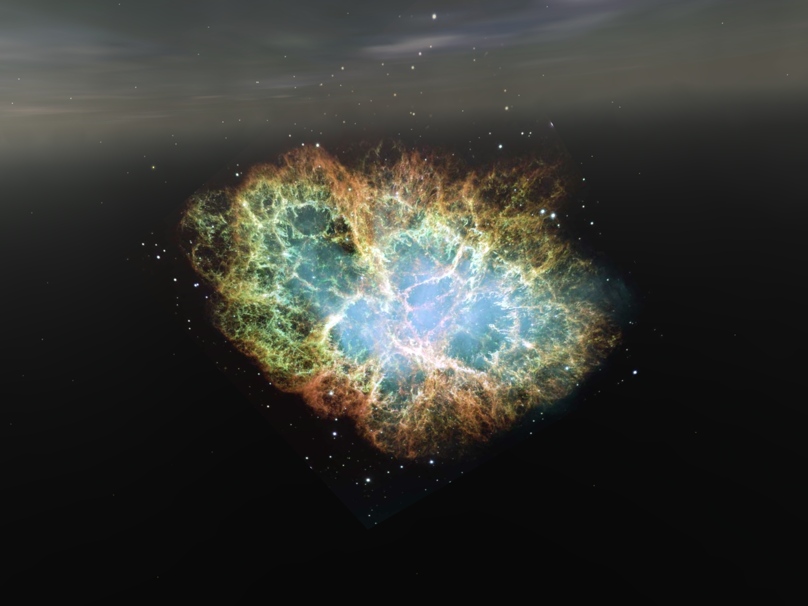
Our connection to the cosmos is not only through star birth, but also via the death of stars. Here is the Crab Nebula, the remnant of a supernova that was observed by Chinese and Arab astronomers and no doubt the American Indians in 1054 AD.

A supernova is the explosive death of a massive star. Except for hydrogen and helium, almost every other element has been forged inside a star. This includes the carbon, oxygen, and nitrogen that are found in organic molecules and every other element heavier than those.

The supernovae explosions disperse these elements across the galaxy, where they can become incorporated in the next round of star and planet formation. We and everything we are familiar with are literally made up of star-stuff, elements that have been processed in the interiors of stars

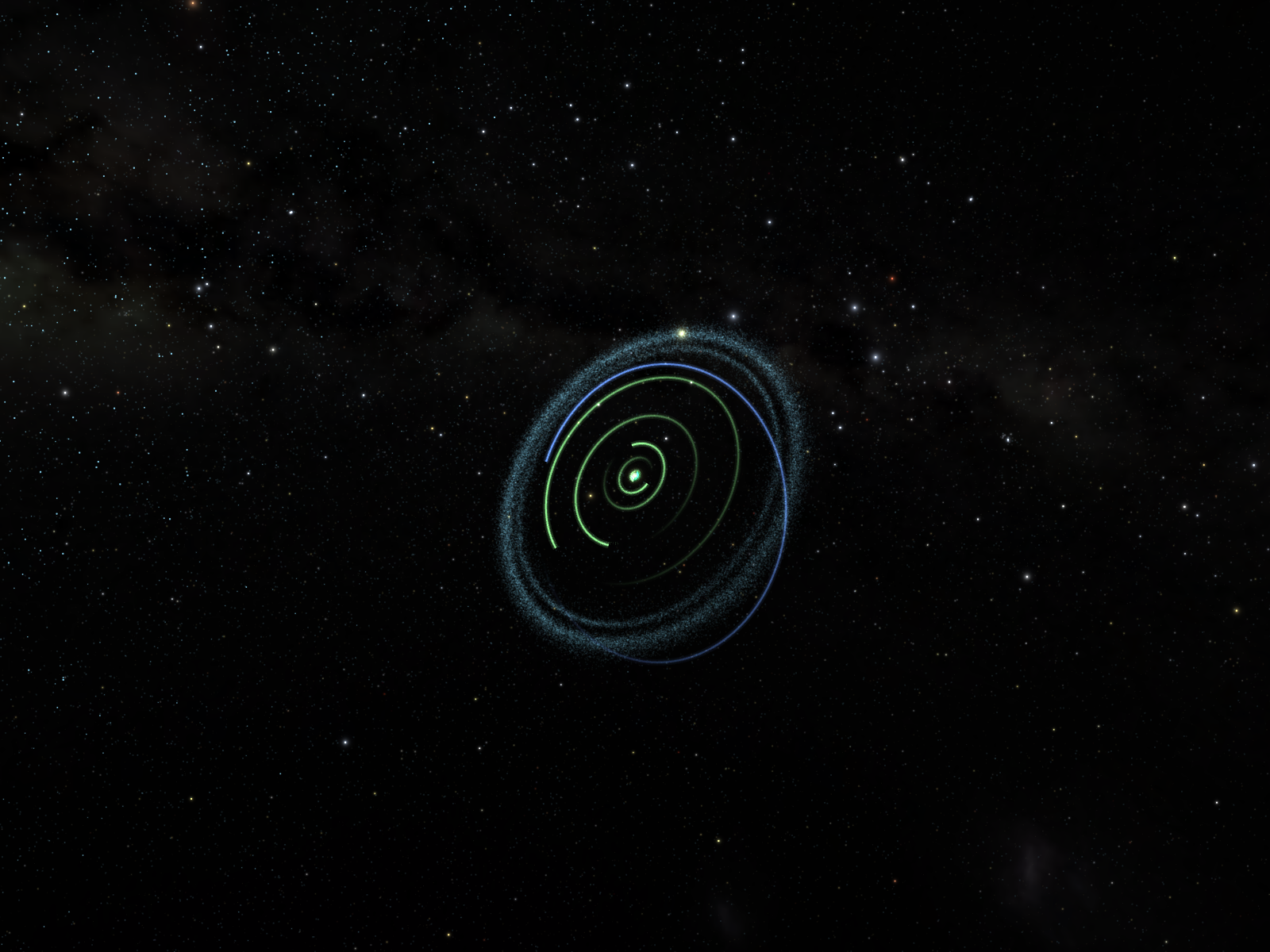
As we near the Sun, we fly through the Oort Cloud, a spherical shell of several trillion icy comets. Then we see the Kuiper Belt, a toroidal band of several billion icy bodies that lie outside the orbits of Neptune and Pluto. These are the remnants of planet formation, leftover debris from the early Solar System.

These bodies, along with many icy moons of the outer planets, contain substantial amounts of water – more than 99% of the water in the Solar System. But the water here is frozen, and inaccessible to life.

When we get into the inner Solar System, we see a visualization of its habitable zone, the region where liquid water can exist on the surfaces of rocky planets.

Note that the Earth is right in the middle of the zone.

We think that Earth, Mars, and Venus actually started with similar conditions early in the Solar System’s history. However Mars’ and Venus’ locations at the outer edges of the habitable zone has allowed both of them to dry out. Mars has evolved into a cold dusty desert world, while Venus has a surface hot enough to melt lead.

Our voyage through the cosmos returns us back to the Earth, a blue marble that is an island in the sea of space. It has just the right conditions, with sufficient water, atmosphere, and active geology that has allowed life to evolve, persist, and thrive for billions of years. It has been, and for the foreseeable future, will be our only home in the Universe.

We are part of the first generation to be able to view the Earth in total from the vantage point of space.

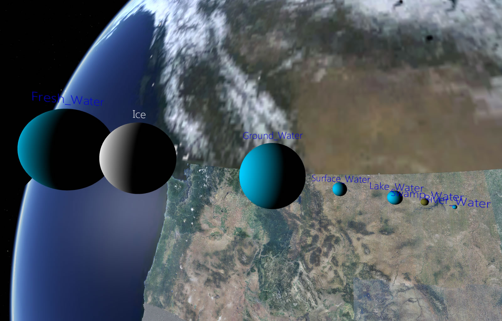
All of the water on earth has a volume that would fill a cube with sides of 1,150 kilometers, that is 713 miles. The cube would cover the state of Montana and reach nearly three times the height of the International Space Station’s orbit. Seventy one percent of the earth’s surface is covered by water and only 2.8% of the water volume on earth is fresh water. If the large sphere is the total volume of fresh water on earth we can now describe what makes up the precious resource. Seventy-five percent of the fresh water is in the form of ice and an additional 20% is in ground water. The remaining 5% the fresh surface water is distributed in lakes, swamps, and rivers. The final very small segment of our earth’s water resource in water vapor in the atmosphere that make up only .04% of the total fresh water and is the fuel that drives our weather.

This presentation will focus on the mechanisms here on earth and more specifically here in the Black Hills of South Dakota that result in the distribution water on the surface of the planet, from a continental scale, from a regional scale in the western part of North America, and then in our Black Hills region South Dakota. The primary message is that within the global water cycle there are times when in isolated locations, extreme conditions can be very destructive.

The habitable zones of the Earth are small, and precious. Each one of them has a supply of potable water.

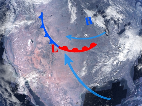
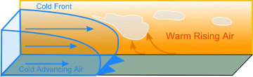
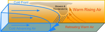
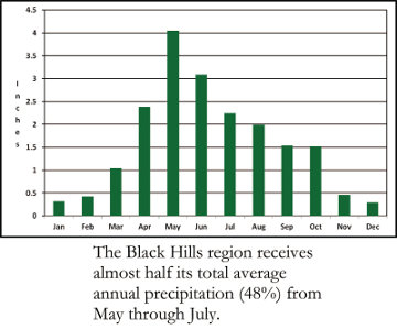
In the simplest terms our weather is driven by temperature and moisture. In the Black Hills our moisture comes from the Gulf of Mexico and the Great Lakes. During late spring and early summer the great plains will often have conditions where a cold dry arctic air mass will move southward while a warm moist air mass will move up from the Gulf of Mexico and along that boundary, called a front. As the front advances, the colder air lifts the warmer air ahead of it. The air cools as it rises and the moisture condenses to produce clouds and precipitation ahead of and along the cold front. In contrast to lifting along a warm front, upward motions along a cold front are typically more vigorous, producing deeper clouds and more intense bands of showers and thunderstorms. However, these bands are typically quite narrow and move rapidly just ahead of the cold front. Weather forecasters can predict the likelihood of rain by measuring the air temperature to dew point spread; the closer the dew point temperature is to air temperature the greater the moisture saturation and therefore increasing the chance of producing rain or snow. Nearly all of our moisture in the Black Hills region occurs due to this type of rain event and generally in the late spring and early summer - as depicted on this bar chart.

Terrain is another factor that can influence our weather. The formation of the Black Hills occurred during the same geologic time as the Rocky Mountains. Over many hundreds of millions of years and through multiple inundations of inland seas layers sedimentary rock were deposited on the igneous rock core. Toward the end of the Cretaceous, or about 65 million years ago, the Black Hills were thrust up during a period of mountain building. At that time the highest elevations were probably over 14,000 feet above mean sea level. Over time, this uplifted dome was eroded down to its present elevation with the highest peak at 7,244; the highest peak between the Rocky Mountains and the Swiss Alps. The Black Hills are an “island in the plains” which are sacred to the American Indians and also affects the weather of our area due to rising terrain in an otherwise flat prairie.

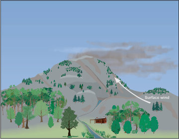
In geography, the term 'orographic effect' refers to the weather condition triggered by upward movement of an air mass coming in contact with a mountain or some other elevated terrain.

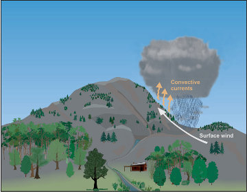
When the air mass moves over a rising terrain, it is automatically forced to move upwards. This upward movement of air mass triggered by rising terrain is referred to as the 'orographic lift'. As the mass of air continues to rise, it is subjected to adiabatic cooling - cooling of a body of air without the addition or subtraction of heat or thermal energy. This phenomenon - wherein temperature decreases as altitude increases, eventually results in condensation of air. When relative humidity is at 100 percent, it triggers cloud formation resulting in precipitation - which is referred to as 'orographic precipitation'. These storms that originate in mountainous areas will generally move off into the plains due to the higher winds at altitude.

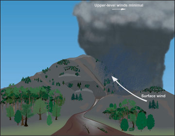
While this explains the increased likelihood of afternoon thunderstorms building over the Black Hills, it does not explain the storms that caused the flooding in 1972. On those rare occasions when thunderstorm activity caused by orographic lift is also accompanied by very light winds at altitude, the storms become anchored and/or move very slowly causing localized heavy precipitation. In the Black Hills, this slow movement, down slope, along the stream drainage systems will result in flash flooding.

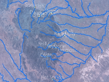
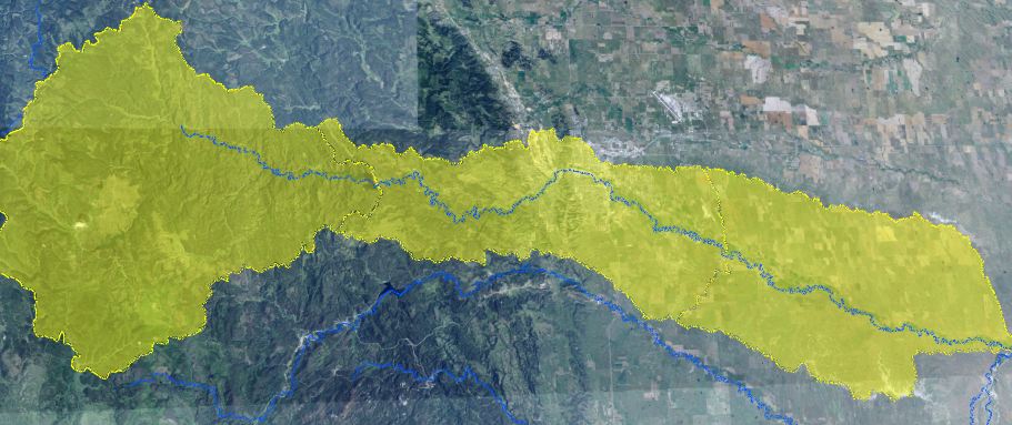
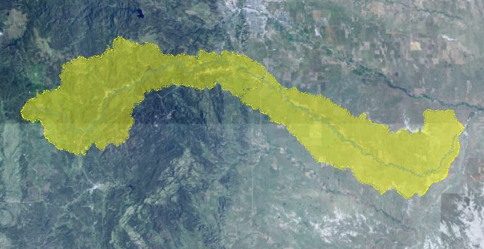
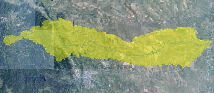
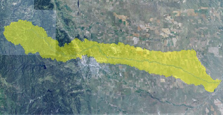
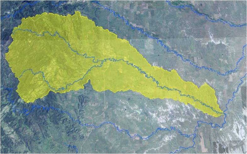
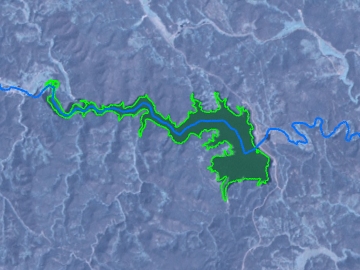
We can see the major rivers and streams of the Black Hills region now and with the help of the USGS South Dakota Water Science Center we have included the total watershed areas for these rivers and streams. We’ll turn on the labels for the major towns in the Black Hills to help orient you.

On June 9, 1972 the unusual and excessive rainfall was the result of a strong low-level easterly air flow that forced moist air upslope over the hills. This sustained orographic effect helped the air to rise, cool, become very unstable, and release its moisture in repeating thunderstorms. Another important contributing factor was the unusually light winds at higher altitude. These light winds did not disperse the moist air or move the thunderstorms along to prevent the extreme concentration of rainfall. Instead, these conditions allowed heavy rainfall to remain almost stationary along the eastern slopes of the Black Hills. The first reports of significant rainfall were at 3:00 p.m. and by 6:00 p.m. there was a solid line of storms from Sturgis to Keystone on a line east of Pactola Dam which remained stationary until slowly moving eastward beginning about 10:00 p.m. In Rapid City the heaviest rain continued until approximately midnight with light rain falling until 4:00 a.m. on June 10th.

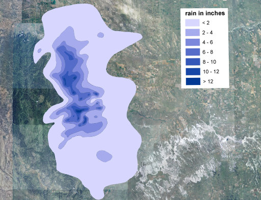
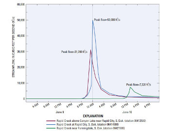
The Uniview image you now see includes the stream watershed areas for the eastern Black Hills and overlaying this we have turned on the isohyetal map showing the lines of equal rainfall during the 12 hour period on June 9 & 10. The levels are represented by differing shades of blue with the darkest representing 14 inches of rainfall to the lightest at 2 inches . As you can see the heaviest rainfall fell between Pactola and Rapid City on a line from Sturgis to the north and Keystone to the south. The worst flooding occurred on Rapid Creek, Spring Creek, Box Elder and Battle Creek. On Rapid Creek, the total drainage area above Canyon Lake is 371 square miles; however, just 14% of this area or 51 square miles of drainage downstream of Pactola Reservoir contributed to the flood runoff into Rapid City. The peak discharge on Rapid Creek just above Canyon Lake was 31,200 cubic feet per second, while the discharge from Pactola never exceeded 74 cfs, the normal discharge from the dam.

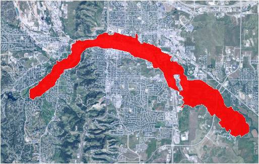
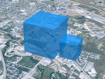
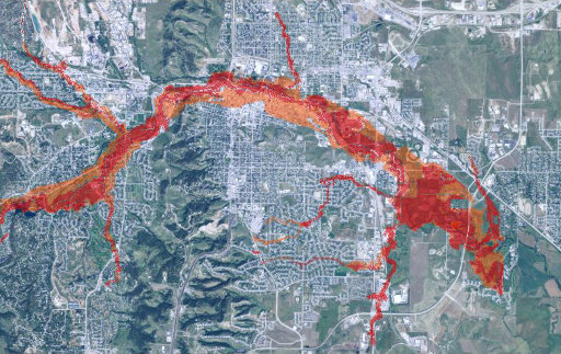
At approximately 10:00 p.m. water began to flow over the spillway on Canyon Lake with creek levels increasing 12 feet between 9:15 and 11:15 p.m. The gates on the spillway were opened to lower the level but were soon clogged with debris. The water level continued to rise and soon overtopped the entire dam. Although the main break in the dam probably washed out fairly rapidly, it was reported that water flowed over the top of the dam for approximately 45 minutes before the dam gave way at 10:45 p.m. The peak flow of 12,500 cfs from Cleghorn Canyon just above Canyon Lake coincided with the breaching of the dam. The total of these two flows accounts for 86% of the estimated peak flood in Rapid City of 50,000 cfs along Omaha Street. The size of Canyon Lake compared to the flood flow along Rapid Creek over and through the lake is minimal; however when the dam did fail it likely added to the 50,000 cfs rampage, resulting in additional loss of life. This image shows the boundaries of the 1972 flood from Canyon Lake through Rapid City. The area of the flood is depicted in this layer in red; and to provide some perspective on the amount of water flooding Rapid City on that night the next layer compares the volume of Pactola Reservoir in the near square mile to the flood waters in the taller square mile patch - the equivalent of 14.5 Pactola volumes flooded Rapid City.

The flood resulted in 238 people killed, 8 of the deaths in Keystone and 3,057 were injured, including 118 who needed hospital care. Six months after the flood, eight people were still listed as missing. The flood caused $160 million in damage equal to $905 million in 2012 dollars; including $37 million in residential property damage and $33 million to businesses and industries. Of the over 1,800 houses flooded, 1,335 were destroyed. Nearly 50 businesses and 5,000 cars were also destroyed.

The response to the flood by local, county, state and federal agencies and non-governmental agencies was swift, compassionate and effective. The SD National Guard was preparing for their annual summer camp on that Friday afternoon and were able to fully mobilize within hours of the Governor’s orders. The NWS issued flash flood warnings at 7:15 p.m. and local off duty police, fire and emergency services were mobilized by the Mayor at 7:30 p.m. Hundreds of responders worked tirelessly over the next few days on rescue and recovery and for some rescuers making the ultimate sacrifice, dying while trying to save others.

Much has changed as a result of this tragedy and others regarding community planning and disaster preparedness. The Federal Emergency Management Agency was established to coordinate federal resources during a response and assist local and state planners to prepare for such disasters.

For the purposes of public safety and community planning, FEMA has developed Flood Maps showing where historically flooding has and will occur. Based on the probability and intensity of flooding, FEMA uses a 100 year flood prediction that becomes the basis for community planning. These high risk areas have a 1% annual chance of flooding and a 26% chance of flooding over the life of a 30-year mortgage. Areas of moderate flood hazard, usually the area between the limits of the 100-year and 500-year floods.

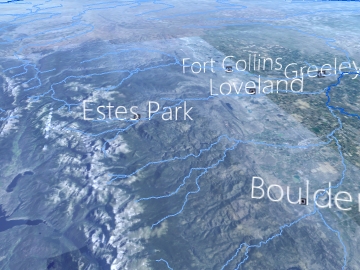
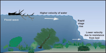
At the time little was know about the history of such a devastating flood, there was nothing to compare it to. The magnitude was greater than any previous flood; until the Big Thompson flash flood upstream of Loveland, Colorado on July 31, 1976. This storm was essentially an exact replay of the Black Hills storm. Eight inches of rain fell in one hour-long stretch, and turned the normally placid two-foot-deep trickle into a raging torrent of water 19 feet high. Sweeping 10-foot boulders in front of it, the wall of water sped down the canyon slope. Cars, campers, and buildings in its path had no chance of survival - 145 people were killed.

Much has been learned since then. In fact the US Geological Survey Office in Rapid City recently completed a study of flooding in the Black Hills using the evidence of flooding in caves and ledges in the canyons along critical streams in the Black Hills. The sedimentary evidence from these sites has been dated and the record of flooding is now extends back 2,000 years. In this record are at least 12 events that exceeded the 1972 flood. Two events on Rapid Creek, one approximately 1,000 ago was in the range of 64,000 - 128,000 cfs and the worst event approximately 440 ago was 128,000 - 256,000 cfs; at least 4 times larger than the 1972 flood. This study, published in 2011, was that basis of the Journey Museum’s Mega-Flood exhibit last summer on the 40th anniversary of the 1972 flood. We featured the results of this study and critically important information from the Rapid City and Pennington County Emergency Management Office regarding preparedness and warning.

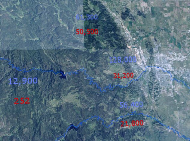
We have put the isohyetal map back up on the screen, I would like you focus your attention on the white numbers above the red on various locations. These represent the peak flows of 1972 in red and the paleo flooding evidence in white.

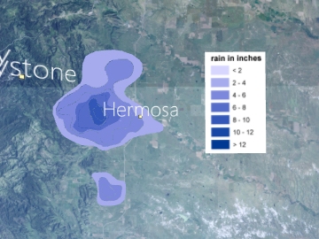
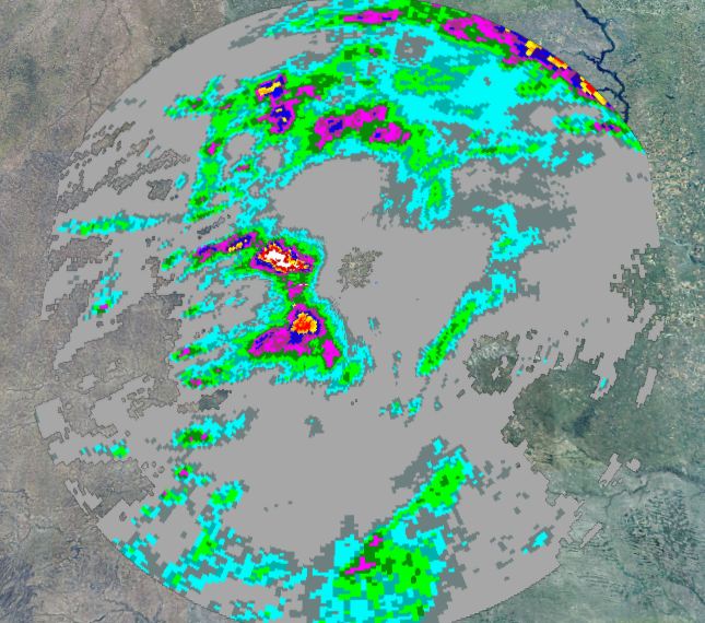
The study revealed that in the context of the now two thousand year record of flooding, we learned that the 1972 flood was not remarkable. That many equal and larger events have occurred before; and in fact, on August 16, 2007 a major thunderstorm with characteristics nearly identical to previous large storms produced rains of over 11 inches west of Hermosa and large sized hail west of Piedmont. The heavy rain fell on the watershed of Battle Creek and Grace Coolidge Creek producing damaging floods in Hermosa. Today’s radar technology is much advanced over what was available 40 years ago. As a forecast tool Doppler radar can, in real time determine the intensity of the rain, the presence of hail and velocity of the winds. This provides the forecaster at the National Weather Service with the information to much more accurately predict and track the possibility of flash floods. The next six images you will see are a time lapse of the growth of this storm from 9:00 a.m. to midnight on August 17, 2007. Each successive sweep of the doppler radar provides a cummulative rainfall record.

Paleo floods: 1972 flood isn’t as bad as it gets; it can be far worse.

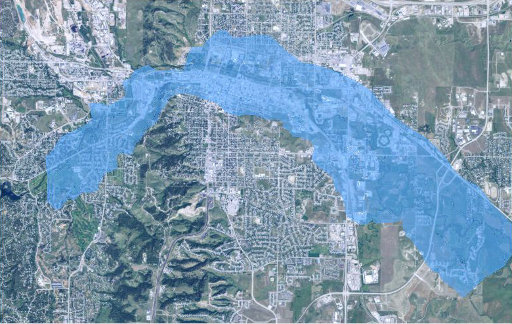
So what do we do now -- we know that we have had major flooding in our lifetime, we learned that floods occurred before recorded time. and can assume that given the amount of erosion we can see all around us that wind and water erosion have sculpted the Black Hills. We must be prepared for future flooding like the 1972 event and know that if a “mega” flood were to occur it would be much more devastating. Here are the 1972 flow rates on various stream in red numbers with the blue numbers representing the estimated paleoflood rates. It is nearly impossible to predict with any real accuracy what such a flood would look like; however, given the flow rates of the flood of 440 years ago the boundaries that would result in Rapid City are estimated in this layer in Uniview. As you can see nearly all of western and central Rapid City would be involved.

We have provided a lot of information in this presentation, some of it fairly basic while some is almost too difficult to process. It is hard to imagine that a future storm could be worse than 1972; but there is much we can and should do.

In 1972 the capabilities to detect and warn the public of the dangers and notifications to evacuate were limited. The NWS did not have a dedicated weather radar, relying on the Ellsworth AFB which was operating intermittently during the storm. The NWS depended on eyewitness reports during the storm and warnings were only sent by TV and radio. The reports to the media were sent via a one-way telephone line with TV and radio reports having copy the verbal report which was read on the air. Only 4 working sirens were available at the time. And worst of all, in 1972 too many people failed to take the warnings seriously and those that did, acted too late and actually became victims. There have been vast improvements in these area have been made through established organizational relationships, communications and technologies.

Now the National Weather Service, in conjunction with the USGS and Pennington County Emergency Management Office work together to provide critical warning information to the public prior to and during severe weather. Weather satellites are used to monitor storms systems, thunderstorm development and atmospheric water vapor to predict the likelihood of severe storms days in advance. Doppler radars now provide detailed images of storm intensity and movements, rainfall rates, and precipitation estimates. Geographic overlays indicate whether the heavy rain is falling in flash-flood prone areas or on saturated soil and where the water is flowing. METWARN is a network of automated stream and precipitation gauges placed along Rapid Creek and its tributaries to provide earlier indication of floods and advance warnings to people along the streams. It was established in the late 1990s as a partnership among the Rapid City/Pennington County Emergency Management Office, the US Geological Survey and the National Weather Service. Weather forecasters monitor the gauge data for heavy rain and flooding and use the data to verify the Doppler radar precipitation estimates, especially in remote areas. NOAA Weather Radio receivers have an alarm to alert people when weather warnings are issued even if they are sleeping, not watching television or listening to the radio, don’t live near a warning siren, or the electricity is off. Emergency Alert System allows local television, radio, and cable TV systems to automatically broadcast warnings from NOAA Weather Radio to their viewers and listeners. And finally, Wireless Emergency Alerts are sent to wireless devices, cell phones and pagers with specific information regarding areas affected by warnings.

These new capabilities will be able to provide timely information to the public in the time of a disaster.

Conclusion & Closing:

Even though we are in what is likely another drought; it is important that we be reminded that these extremely strong storms can happen any year given the right conditions. Its not likely that this would be the year, and it may be many decades before a very large flood happens again; so now is the time to prepare for the worst case. The victims of the 1972 flood paid too high a price; we owe it to them to stay vigilant, make a personal vow to learn more about the warning systems and what to do when notified to evacuate. I would like to turn the program back to David McConville and he will introduce our Public Forum panel of experts.

David ...